Hilbert Curves

When you want to cluster data together over multiple dimensions, you can use Z-Order. But a better algorithm is the Hilbert Curve, a fractal that makes a best attempt to keep adjacent points together in a 1-dimensional space.

From DataBrick's Liquid Cluster design doc we get this graphical representation of what it looks like:

Dotted line squares represent files

A Hilbert curve has the property that adjacent nodes (on the red line, above) have a distance of 1. Note that a property of the Hilbert curve is the adjacent points on the curve are nearest neighbours in the original n-dimensional space but the opposite is not necessarily true. Not all nearest neighbours in the n-dimensional space are adjacent on the curve. How could they be if points have more than 2 neighbours in the original space?

An algorithm in C for navigating this square can be found here. A Python toolkit for handling Hilbert curves can be found here [GitHub]. And a Java implementation can be found here [SO].

The application of this in Big Data is that the data is now sorted. If we were to read through the files following the red line, then each node we encountered is one away from the last. Z-Ordering does not have this property.

Z-ordering. Lines indicate contiguous data. Colours indicate different files.

Unlike the Hilbert curve at the top of this page, there are some large jumps. In fact, the average step is not 1.0 as for the Hilbert curve but 1.557 in this example - over 50% more!

This greater efficiency is true even if we don't take the unlikely case that the data is tightly packed. Below are examples where the data is more realistic and not every possible point (a red +) is actually associated with data (a blue circle).

A Hilbert curve over sparse data

To understand what is going on, we need to appreciate Gray Codes [Wikipedia] which is an alternative numbering system in binary where adjacent numbers only differ by one bit changing (see that parallel with Hilbert curves?). For each bit, for each dimension, we create a mask from the Gray code and do some bit manipulation found here and we'll eventually have a bijective map ℤ^d → ℤ.

The jumps between adjacent data points is less extreme in Hilbert curves. You can see this by-eye if look at a slightly larger space (code here):

A Hilbert curve over sparse data

Typically, the jumps between data points are never more than a couple of positions (average of 1.433). Now, compare this to a similar space using Z-Ordering:

Z-Order over a similar sparse space

and you can see larger jumps between some data points. The average is 2.083 in this run. That's 45% higher than in the Hilbert curve.

Hilbert curves are not currently implemented in Apache Iceberg but are in Databrick's Delta Lake.

Journeys in Data Engineering

I'm currently helping a huge health provider with its data issues. Here are some things I've learned:

Don't bikeshed. There's no point wondering whether you've captured the correct ethnic description ("White? Irish White? Eastern European White?") when there are bigger fish to fry. For instance, hospitals were putting the patients' personal information in the primary key field. This sent the data officer apoplectic until it was cleansed from the files before being sent downstream. But as a result, the downstream keys were not unique. The data scientists consuming this data aggregated it and came to conclusions unwittingly based on one individual having visited the hospital over three million times.

Don't proactively go looking for data quality issues. They'll come looking for you. Continue to build your models but be extremely circumspect. This is a more efficient process than spending time wondering if the data looks good.

Just because the data looks good, it doesn't mean it's usable. How often is the data updated? Is it immutable or is it frequently adjusted? In short, there's an orthogonal axis in data space separate to data quality and it's a function of time. Perfect data that becomes old is (probably) no longer perfect. Perfect data that becomes incomplete is (probably) no longer perfect.

Give a thought to integration tests. Platforms like Palantir are pretty under-developed in this area (answer to my requests for an integration test platform: "we're working on it"). So, you may need to write bespoke code that just kicks the tires of your data every time you do a refresh. 

Remember that documentation is the code. I've had a nice experience using ScalaTest with its Given, When, Thens. It ensured that when running integration tests, the code generated the documentation so the two would never fall out of synch. This is, of course, much harder (impossible?) when running in a walled garden like Palantir.

Stick with a strongly typed language. This can be hard since pretty much all data scientists use Python (and therefore PySpark) but there is nothing worse than waiting several minutes for your code to run only to found out that a typo trips you up. In a language that is at least compiled, such problems would not occur. I'd go so far to say that Python is simply not the correct tool for distributed computing.

Python tools like Airflow are made much easier by using Docker since Python library version management is a pain in the arse. Far better for each application to have its own Docker container.

Never forget that your schema is your data contract as much as an API is your coding contract. Change it, and people downstream may squeal.

Persisting intermediate data sets hugely help debugging. 

Finally, don't use null to indicate something for which you know the meaning. If, for instance, when a record is in a certain state, it's better to say value X equals a flag to indicate that. If you use null, somebody reading that data doesn't know if the record is in this state or if the data is just missing.

Optimizing Spark/DataBricks in Azure

We have about 1.5TB of parquet data in Gen 2 storage on Azure and we're trying to read it with a DataBricks cluster of 8 nodes each with 56gb and 16 cores. All I'm trying to do is some basic select('aColumn).distinct and where('anotherColumn < X).count()s.

Surprisingly, this is running like a dog: the first query takes about 50 minutes and the second about 18. Tuning is an empirical science but this felt wrong as 1.5TB of data is not that much these days.

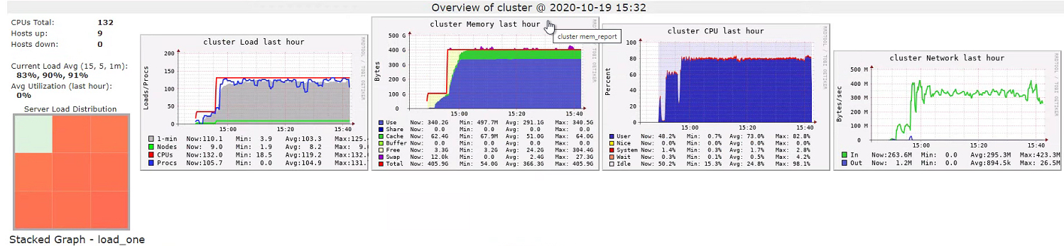
Ganglia Metrics

Ganglia showed that the cluster was running at high capacity although the network usage seemed low. If this is showing the data being pulled from Gen2 into Spark workers, at 300mb/s it would take about an hour to pull it all out of storage. Indeed, this is roughly how long it took. 

However, when I took thread dumps, the executor threads were not waiting on IO. Typically, they were in Spark's CompressibleColumnBuilder (which, according to the docs, "builds optionally compressed byte buffer for a column"). So, it seemed that the cluster really was CPU-bound on parsing the files and garbage collection - which was bad but not horrendous:

Spark GC logs

Calling cache() on the data didn't seem to make queries much faster. Looking at the thread dumps again showed the threads spending a lot of time in CompressibleColumnBuilder for the initial select distinct and in java.io.FileInputStream for the subsequent counts. 

Remembering that  persisting with a storage level of MEMORY_AND_DISK_SER had given me a quick win in the past, I thought I'd try it again but with no success.

I tried enabling the Delta Cache. This is supposed to cache the Gen2 data in the cluster:

Storage Tab

Compare this to the storage tab when we're not using Delta Cache and you'll see there won't be any data in the "Parquet IO Cache". (Note that the page says "RDDs" when we're only using the Dataset API. This is standard). Anyway, enabling Delta Cache seemed to make no difference at all.

Using a "Delta Cache Accelerated" cluster actually made the initial distinct.count() take much longer (1.47 hours) with only marginally reduced time for the next query (16.8 minutes).

Disk is incredibly slow compared to memory. Ultimately, I was trying to process too much data with too little RAM and there's only so far tuning will get you before your metrics plateau. So, I made a cluster of 25 nodes each with 28gb of RAM and 8 cores. This did help but not as much as I was expecting. The distinct.count() now took 38 minutes and the where(...).count() 12 minutes. This is between a 25%-33% improvement but still seems a long time in absolute terms.

I want my Data Locality 

The problem appears to be that all the data is pulled to the executors even if we're only interested in just one column [see StackOverflow]. Evidence for this came from another look at Ganglia:

Ganglia Metrics during second query

This was taken after the distinct.count() and during the where(...).count() query. Note that there is no more network activity, suggesting the first query cached the data.

"In Azure really fast networks compensate for having data and compute separated." [ibid] Indeed, the threads seemed to spend all their time on the first call in code to parse the Parquet rather than blocking on IO. But you can't get over the fact that my two queries are doing much the same thing (no joins) but the first takes three times longer than the second. To demonstrate, instead of two different queries, I ran the distinct.count() query twice. The first time took 42 minutes, the second 15. So, it appears that pulling 1.5TB of data from Gen2 into Spark takes about 25 minutes.

Azure is not the only cloud offering that implements this architectural trick. GCP takes all the data out of storage and puts it into an ephemeral HDFS cluster.

Solution

A new day, a new dawn. Let's start the cluster again and go from the beginning. This time, I won't explicitly enable IO cache and I won't even call .cache() on my DataFrame. To my amazement, the same query ran in about 30 seconds today! It seemed that this .cache() call was the root of my problems as re-introducing it returned us to a 50 minute wait. This is pretty much the opposite of what you'd expect with an on-prem Hadoop/YARN cluster.

Spark Gotchas

Some miscellaneous notes on Spark I've been making the last few weeks.

Triggers and OutputModes when Aggregating

I was experimenting with aggregating a query that reads from Kafka and writes Parquet to HDFS.

The interplay between watermarking, Trigger and OutputMode look a bit like this:

• Queries that aggregate with OutputMode.Append yet with no watermark will always throw "Append output mode not supported when there are streaming aggregations on streaming DataFrames/DataSets without watermark;;" irrespective of the Trigger. 
• Queries that aggregate with OutputMode.Complete  with "Data source parquet does not support Complete output mode;". Even text files will barf with "Data source text does not support Complete output mode;".
• Queries that aggregatie with OutputMode.Append but with a watermark behave like this:

Trigger	Behaviour
Continuous	Unknown type of trigger: ContinuousTrigger(5000) [1]  or Continuous processing does not support EventTimeWatermark operations.;;
ProcessingTime	No errors but last batch is not pulled from Kafka
none ("When no trigger is specified, Structured Streamin stats the processing of a new batch as soon as the previous one is finished." - Stream Processing with Apache Spark)	No errors but last batch is not pulled from Kafka
Once	No errors but nothing is pulled from Kafka. Running the query twice with awaitTermination pulls some elements.

The reason Spark leaves a little something on Kakfa is (apparently) for efficiency. There appear to be a pull request for making Spark consume the last bit from Kafka but in its associated Jira somebody mentions my StackOverflow question that talks about Spark's behaviour being unchanged.

So perplexed was I that I asked the Spark mailing lists. The answer from Spark committer, Jungtaek Lim, was illuminating:

"Unfortunately there's no mechanism on SSS to move forward only watermark without actual input, so if you want to test some behavior on OutputMode.Append you would need to add a dummy record to move watermark forward."

This doesn't seem to be because we're writing Parquet. Text files will also behave this way.

Defragging Question

Spark will create a new file per executor thread per ProcessTrigger time (as this test code demonstrates). This can lead to a lot of files that could ultimately choke your Name Node if you're persisting to HDFS. This may necessitate a roll-your-own fix [SO].

If you're using DataBricks, you can do this "bin-packing" by running the OPTIMIZE command. Unfortunately, I could not see the code to do this inside the Delta library DataBricks have open sourced. (I discuss other ways of dealing with this problem without Delta in this blog post).

Since our use case at work is such that we only want the output of stream processing once a day, we opted for Trigger.Once. Since we're not aggregating, all of the data is pulled and processed. Since this is streaming in a very loose sense of the word (it's more batch processing that gets its data in one short, sharp stream), we avoided having large numbers of small files.

Exceptions in processing DataFrames

Spark can optionally have a "best efforts" approach to exceptions rather than failing the whole process.

spark.range(10000).repartition(7).map { i =>
  if (i == 9999) { Thread.sleep(5000); throw new RuntimeException("oops!") }
  else i
}.write.option("mapreduce.fileoutputcommitter.algorithm.version", ALGO_VERSION).mode("append").parquet(s"/tmp/test_algo_$ALGO_VERSION")

When ALGO_VERSION=1, nothing is written to HDFS. On the other hand, when ALGO_VERSION=2, the partition in which the exception occurred is not written but all the other ones are.

see https://databricks.com/blog/2017/05/31/transactional-writes-cloud-storage.html

DataFrame types

You can see the schema as JSON with:

spark.read.parquet("THE_FILE").schema.json

The type "timestamp" would map the data to a java.sql.Timestamp (the equivalent of a SQL TIMESTAMP type). This Java type is a subclass of java.util.Date.

The type "date" would map to a java.sql.Date (the equivalent of a SQL DATE type). This is also a subclass of java.util.Date.

See this StackOverflow page  for descriptions of the SQL types.

Trying to read from a Parquet file that uses "date" and coercing it to a "timestamp" will result in:

Caused by: java.lang.UnsupportedOperationException: org.apache.parquet.column.values.dictionary.PlainValuesDictionary$PlainIntegerDictionary

Idempotency

DataStreamWriter.foreachBatch is experimental and "is supported only the in the micro-batch execution modes (that is, when the trigger is not continuous)". It provides a batchId that "can be used deduplicate and transactionally write the output (that is, the provided Dataset) to external systems. The output Dataset is guaranteed to exactly same for the same batchId (assuming all operations are deterministic in the query" [Spark docs].

[1] "You can set the optional Continuous Trigger in queries that satisfy the following conditions: Read from supported sources like Kafka and write to supported sinks like Kafka, memory, console." SO quoting DataBricks.

Zeppelin 1

Introduction

When I'd tinkered with Zeppelin in the past, it seemed a bit buggy but using zeppelin-0.8.1-bin-netinst has been reasonably straightforward.

The reason we want to get it into my current project is that the analysts want to play with and visualise the data without getting to close to Spark.

Configuring

I had to add dependency:

org.apache.commons:commons-lang3:3.5

to the Spark interpreter (see StackOverflow) because I was getting:

Caused by: java.io.InvalidClassException: org.apache.commons.lang3.time.FastDateParser; local class incompatible: stream classdesc serialVersionUID = 2, local class serialVersionUID = 3

when trying to call Spark. I also added the properties:

HADOOP_CONF_DIR
HADOOP_HOME   
SPARK_HOME

to the interpreter config in the web admin GUI and

export MASTER=yarn-client
export HADOOP_CONF_DIR=/media/sdb8/Tools/Cluster/Hadoop/Current/etc/hadoop/
export SPARK_HOME=/media/sdb8/Tools/Cluster/Spark/Current/

to ZEPPELIN_HOME/conf/zeppelin-env.sh.

I also set up Hadoop again (following my own advice here) but this time I had to unexpectedly tweak the config as my secondary name node was trying to contact 0:0:0:0. It required defining dfs.namenode.secondary.http-address in hdfs-site.xml (see StackOverflow) and my problem went away.

Running

Gratifyingly, I got:

To add your own code to the classpath by setting spark.jars to your uber-jar (see the documentation).

Lo and behold, we can now use Zeppelin to ask Spark to calculate trigrams on a corpus using code I'd written elsewhere:

Note, to then use PySpark and all the libraries you've installed with pip, you'll want to set the zeppelin.pyspark.python property in the Spark interpreter (not the zeppelin.python property in the Python interpreter) and un-tick zeppelin.pyspark.useIPython. Otherwise, all those Python libraries you've installed won't be found.

Addendum (23/5/2019)

After a few weeks of playing with Zeppelin, I'm still pretty impressed despite a few glitches in the GUI. However, it's still annoying that I cannot push/pull to a Git repository. And I got bit by this (StackOverflow) too,

It's also worth mentioning that if you're running Zeppelin on a headless server (like AWS), you will need to follow the instructions here if you want some of Python's wonderful graphics libraries.

FP and Big Data part 2

Functional Programming gives guarantees that Big Data tools can leverage. For example, in the event of an aggregation, "such as SUM, expressible as an associative and commutative operator (who said “monoid”?), it can be executed more efficiently, e.g. the framework can push some aggregation into the first map. In Hadoop, such an aggregation is called a combiner." (Eugene Kirpichov at Medium.com)

Note that Spark's [SO] reduce (and indeed Scala's too) is over commutative semigroups when it should be on just semigroups. "The class of commutative semigroups consists of all those semigroups in which the binary operation satisfies the commutativity property that ab = ba for all elements a and b in the semigroup." (Wikipedia).

[In Scala, "reduceLeft and foldLeft apply the operator from left to right (head to tail). reduceRight and foldRight apply it from right to left. As for reduce and fold, the order is unspecified, which is what allows to have parallel implementations for it (see ParIterableLike). As a consequence, you'd better be sure that your operator is associative [and commutative - think String concatenation] when calling reduce, otherwise the result will not be deterministic." (StackOverflow)]

This clearly is not true for some obvious semigroups (for instance, string concatenation with the empty string being the "zero" element). But it's not necessarily true for Java primitives either.

Haskell doesn't have an issue with floating point folding:

$ ghci
GHCi, version 7.10.3: http://www.haskell.org/ghc/  :? for help
Prelude> foldr (\x y -> x + y) 0 [1.0, 0.05, 0.05]
1.1
Prelude> foldl (\x y -> x + y) 0 [1.0, 0.05, 0.05]
1.1

Whereas, Scala (due to the IEEE754 standard) gives this:

    val floats = Seq(1.0f, 0.05f, 0.05f)
    println(floats.sum)                 // 1.0999999
    println(floats.reduce(_ + _))       // 1.0999999
    println(floats.reduceLeft(_ + _))   // 1.0999999
    println(floats.reduceRight(_ + _))  // 1.1

And it's not just floating point arithmetic that has this problem. If you exceed the maximum value for the Integer and Long, you also will suffer misery.

So be careful. Certain FP rules are not enforced in the JVM.

Hive

I'm building a Hadoop ecosystem test harness that will allow a whole slew of applications to be tested in a single JVM, in a single integration test (source).

A test for this harness fired up Zookeeper, Kafka, HDFS, Spark and finally Hive. It feeds Kafka with messages and Spark Structured Streaming processes them writes them as Parquet to HDFS. Finally, Hive reads this file and checks that what it reads is what Spark processes.

This all works fine until I decided to partition the Spark DataStreamWriter. Then, Hive didn't see any data and the the test failed upon an assertion that what Spark sees, Hive sees. Annoyingly, the test did not fail because of what is essentially misconfiguration. The reason being that Hive keeps a store of meta data about all the things it can see and although the data is there to be read, it's not been told to do so until the metastore is updated.

So, putting a long Thread.sleep in the test code I then fired up Beeline with something like:

beeline> !connect  jdbc:hive2://localhost:40327/default

whereupon we're asked to enter a user name and password. First, we recognize the data:

0: jdbc:hive2://localhost:40327/default> create external table parquet_table_name (key String, value String) PARTITIONED BY (partitionKey Date)  STORED AS PARQUET LOCATION 'hdfs://127.0.0.1:33799/tmp_parquet/';

No rows affected (0.077 seconds)

but we can't see any rows:

0: jdbc:hive2://localhost:40327/default> select count(*) from parquet_table_name;

No rows selected (0.204 seconds)

+------+

| _c0  |

+------+

| 0    |

+------+

This seems to be because there are no partitions:

0: jdbc:hive2://localhost:40327/default> show partitions parquet_table_name;

+------------+

| partition  |

+------------+

+------------+

No rows selected (0.219 seconds)

The solution was to add the partitions manually:

1: jdbc:hive2://localhost:40327/default> ALTER TABLE parquet_table_name ADD PARTITION (partitionKey='2018-11-28') location 'hdfs://127.0.0.1:33799/tmp_parquet/partitionKey=2018-11-28/';

No rows affected (0.155 seconds)

1: jdbc:hive2://localhost:40327/default> show partitions parquet_table_name ;

No rows affected (0.327 seconds)

+--------------------------+

|        partition         |

+--------------------------+

| partitionkey=2018-11-28  |

+--------------------------+

Contrary to the advice I read elsewhere, MSCK REPAIR TABLE parquet_table_name  SYNC PARTITIONS;  did not seem (because of camel-case names) to help me (the command ALTER TABLE table_name RECOVER PARTITIONS; seems to be just for Amazon's version of Hive).

Now, counting the rows gives me (some of) my data:

1: jdbc:hive2://localhost:40327/default> select count(*) from parquet_table_name;

+-------+

|  _c0  |

+-------+

| 2879  |

+-------+

1 row selected (1.939 seconds)

I'm not a Hive expert so there may be a solution that just adds anything in the directory (despite all the advice on forums, I could not get that to work the column name on which it's partitioned needs to be lowercase and mine was camel case). However, this hack works for now.

There appears to be a JIRA to make this automatic but there is nothing at the moment.

Parquet tuning

I watched Ryan Blue's excellent "Parquet Performance Tuning" video (here and slides here). But before watching it, it's worth familiarizing yourself with the glossary at the Parquet github page:

Row group: A logical horizontal partitioning of the data into rows. There is no physical structure that is guaranteed for a row group. A row group consists of a column chunk for each column in the dataset.

Column chunk: A chunk of the data for a particular column. They live in a particular row group and are guaranteed to be contiguous in the file.

Page: Column chunks are divided up into pages. A page is conceptually an indivisible unit (in terms of compression and encoding). There can be multiple page types which are interleaved in a column chunk.

Hierarchically, a file consists of one or more row groups. A row group contains exactly one column chunk per column. Column chunks contain one or more pages. The units of parallelization are:

Job	Granularity
MapReduce	File/Row Group
IO	Column chunk
Encoding/Compression	Page

Tuning Parquet

My notes from the video are:

• Parquet builds a dictionary and "just stores pointers into that dictionary ... basically the big trick in Parquet compression". 
• Dictionaries not only save space but can be used for filtering (no entry means that data page doesn't have it). It is highly recommend to implement data locality as it leads to smaller dictionaries.
• Be careful of writing too many files (22'18"). Incoming partitions are not the same as outgoing partitions. That is, the partition key on the incoming file need not be that of the outgoing.
• Look at CPU usage and bytes read not wall time as that can vary (just plain stats).
• Use parquet-tools to see the stats demonstrating that your data really is partitioned as you expect and has sensible splits (eg, A-z is wrong but A-F, f-M etc is better).
• Every row group has its own dictionary (43'10").
• Decreasing row group size increases parallelism.
• "You're going to need a sort anyway if you want to take advantage of stats" (46'10"). See below for a further explanation.
• Brotli compression "does really really well with text data" (47'20").

To take advantage of the stats embedding in the files "you need to insert the data sorted on filtering columns Then you will benefit from min max indexes and in case of orc additional from bloom filters, if you configure them.  In any case I recommend also partitioning of files (do not confuse with Spark partitioning)" (see here).

Interestingly, the Parquet documentation has something to say about HDFS block sizes: "We recommend large row groups (512MB - 1GB). Since an entire row group might need to be read, we want it to completely fit on one HDFS block. Therefore, HDFS block sizes should also be set to be larger. An optimized read setup would be: 1GB row groups, 1GB HDFS block size, 1 HDFS block per HDFS file."

HBase, Cassandra and CAP

Which is best - Cassandra or HBase? Well, it depends what you're trying to do.

The oft-quoted comparisons generally involve Eric Brewer's CAP-theorem (the formal proof by Gilbert and Lynch can be found here and an updated review here) and you can see pictures like this dotted around the web:

From "Cassandra: the Definitive Guide" quoted here

(where the RDMBS offerings imply Two-Phased Commit).

Most developers have some awareness of CAP but there are a lot of misconceptions - typically that you can have at most two elements of Consistency, Availability or Partition tolerance - but not all three. "The 2 of 3 formulation was always misleading because it tended to oversimplify the tensions among properties" (from an article by Brewer himself found here).

Allowing at least one node to update state will cause the nodes to become inconsistent, thus forfeiting C. Likewise, if the choice is to preserve consistency, one side of the partition must act as if it is unavailable, thus forfeiting A. Only when nodes communicate is it possible to preserve both consistency and availability, thereby forfeiting P. The general belief is that for wide-area systems, designers cannot forfeit P and therefore have a difficult choice between C and A.

Here are some common misconceptions corrected.

• The C in CAP "has got nothing to do with the C in ACID, even though that C also stands for 'consistency'" [1]. "Gilbert and Lynch use the word “atomic” instead of consistent in their proof, which makes more sense" [2]. The C in ACID has several similar but not mutually exclusive meanings which include not violating any database constraints, linearizability (see below), ensuring the data is consistent (eg, domain-specific rules such as taking X out of one bank account and into another means the total money overall does not change).
• "The CAP model says nothing about transactions that touch multiple objects. They are simply out of scope for the theorem" [2].

In "Please stop calling databases CP or AP", Martin Kleppmann says:

"But if you’re using some other notion of consistency or availability, you can’t expect the CAP theorem to still apply. Of course, that doesn’t mean you can suddenly do impossible things, just by redefining some words! It just means that you can’t turn to the CAP theorem for guidance, and you cannot use the CAP theorem to justify your point of view.

"If the CAP theorem doesn’t apply, that means you have to think through the trade-offs yourself. You can reason about consistency and availability using your own definitions of those words, and you’re welcome to prove your own theorem. But please don’t call it CAP theorem, because that name is already taken."

In the CAP theorem:

• Consistent means Linearizability,  think of visibility in terms of variables in the JVM. "If operation B started after operation A successfully completed, then operation B must see the the system in the same state as it was on completion of operation A, or a newer state." [1] A master that asynchronously replicates to slaves is an example of a non-linearizable system. Note: some systems (eg a DB that uses MVCC) are intentionally non-linearizable.
  
  
• Availability means “every request received by a non-failing [database] node in the system must result in a [non-error] response” [from the proof]. Note, the response can take an arbitrary amount of time which might violate some people's notion of availability...
  
  
• "Partition Tolerance (terribly mis-named) basically means that you’re communicating over an asynchronous network that may delay or drop messages." Which is basically the internet. "
  
  "In practical terms, a distributed system cannot be made immune to network failures... If the system chooses to favor Availability (such systems are designated AP systems), then it will continue to service requests, even though the data could be in an inconsistent state... If the system chooses to favor Consistency (known as a CP system), then it will choose to stop serving requests (become unavailable) if the consistency of data cannot be guaranteed. For a CP system, this is achieved by requiring a certain number of nodes to confirm that a data update has been made before acknowledging the update." [Hazelcast]

Using these definitions, Cassandra is not AP for quorum read/writes. If there is a partition split, the nodes on the wrong side of the split cannot reach a consensus and therefore are not available. (Interestingly, Brewer notes "as some researchers correctly point out, exactly what it means to forfeit P is unclear.")

So, although Cassandra and HBase both have their pros and cons, mentioning the CAP theory is orthogonal.

(Aside: although Elastic Search is a search engine not a database, there is an interesting chat about how CAP applies to it here.)

A solution?

There's a cheekily entitled blog post (it's titled "How to beat the CAP theorem" but in it he says "You can't avoid the CAP theorem, but you can isolate its complexity and prevent it from sabotaging your ability to reason about your systems"). This isolation is via immutability.

In this post, author Nathan Marz talks of DBs "choosing availability over consistency":

The best consistency guarantee these systems can provide is eventual consistency. If you use an eventually consistent database, then sometimes you'll read a different result than you just wrote. Sometimes multiple readers reading the same key at the same time will get different results... It is up to you to repair the value once you detect that the values have diverged. This requires tracing back the history using vector clocks and merging the updates together (called read repair)

Marz' proposal to use immutable data leads us to this conclusion:

If you choose consistency over availability, then not much changes from before. Sometimes you won't be able to read or write data because you traded off availability... Things get much more interesting when you choose availability over consistency. In this case, the system is eventually consistent without any of the complexities of eventual consistency. Since the system is highly available, you can always write new data and compute queries. In failure scenarios, queries will return results that don't incorporate previously written data. Eventually that data will be consistent and queries will incorporate that data into their computations.

This mitigates Brewer's proposal that revolves around reconciliation during a partition recovery phase. Marz' proposes no reconciliation, just a deferred sharing of the data.

[1] Martin Kleppmann's blog.
[2] Julian Browne's blog.

Building Big Data Apps

After spending the last 18 months using Spark to write an entity resolution software for over a terrabyte of data, here are some miscellaneous notes of what I wish I'd known from the start. In no particular order:

1. Make sure your app can recover from a failure easily. Write to HDFS after each major stage. This will also help debugging when the answer that comes out of the sausage machine wasn't entirely what you were expecting. ("Simply split long-running jobs into batches and write intermediate results to disk. This way, you have a fresh environment for every batch and don’t have to worry about metadata build-up" from here). Also, the topology for one stage may not be appropriate for another (see here for an example where smaller numbers of executors with more resources - contrary to the general Spark advice - gives better performance).

2. Small inefficiencies can cause big problems. Use jstack liberally.

3. Don't use Spark as a key/value lookup. That's not what it's built for. Use another system. Don't try to hack it by using a broadcast variable as that simply doesn't scale.

4. Use realistic data, both in size and quality. Making fake data is surprisingly hard if you want the output to remotely correspond to the real world.

5. Have an automated test in a realistic environment (you don't want authentication problems to show up late, for example). Run the app daily in this environment to show any performance changes

6. "Don't start modeling before designing some measurable goals" [1]. Define acceptance criteria early on as to what you'd expect to come out and what you wouldn't. Estimate the false positive/negative rate. For example, at one point we expected 220k of company entities to resolve with Orbis data. Using a very simple query, we were seeing about 130k of our businesses resolve to something. Therefore, the true positive rate could not be higher than about 60% (and may have been less) therefore there was work to do here.

7. Pass small objects around, preferably just IDs. This is what the built-in Connected Component algorithm does. It will improve performance.

The stages of my app

There were 6 stages to my application:

1. Build a matrix using TF-IDF to assign weights to words.
2. Calculate the cosine similarities.
3. Execute bespoke business rules.
4. Find connected components.
5. Turn those IDs back into entities.
6. Consolidate the relationships between these resolved entities in a process called Edge Contraction.

There were some interesting modifications to this basic flow.

1. Feature hashing improved run time performance but the largest connected component went from 600 to 26 000 (BlackRock/Merrill Lynch who seem to have created what appears to be a lot of shell companies with similar names).

2. By ignoring all words that appear in over 1000 documents, there was no need for stop words. This was useful since the corpus was multilingual.

A note on requirements gathering

One tip in finding which database suits you come from the late Dr Jim Gray. "Gray's recipe for designing a database for a given discipline is that it must be able to answer the key 20 questions that the scientist wants to ask of it." [2] A real-world example can be found here. The idea being that 20 questions is the roughly the minimum number of questions you need before a pattern emerges.

This teased out of the business that we needed more than just a graph database (like Neo4J) which they seem for some reason to have fixated on at one point. We also needed the batch processing that GraphX gave us.

[1] Practical Data Science with R.

[2] The Fourth Paradigm: Data-Intensive Scientific Discovery, Tony Hey.

Playing with Pregel

Implementing your own distributed Pregel algorithm in GraphX is surprisingly simple but there are a few things to know that will help you.

First, what is GraphX's Pregel implementation? Well, it takes three functions:

1. one that merges messages of type T, that is (T, T) => T.

2. one that runs on each vertex with an attribute type of VD and that takes that message and creates a new state. Its type is (VertexId, VD, T) => VD.

3. one that runs on each edge/vertex/vertex combination and produces messages to be sent to the vertices. Its type is (EdgeTriplet[VD, ED]) => Iterator[(VertexId, VD)] where ED is the edge's attribute type.

TL;DR: the vertex holds its state and the edges send it messages. If this starts sounding like the Actor Model pattern to you, you're not alone

"It's a bit similar to the actor mode if you think of each vertex as an actor, except that vertex state and messages between vertices are fault tolerant and durable, and communication proceeds in fixed rounds: at every iteration the framework delivers all messages sent in the previous iteration. Actors normally have no such timing guarantee." - Martin Kleppmann.

So, off I went and wrote my code where all the paths through a vertex are stored as state at that vertex.

And it ran like a dog. After five hours of processing, it died with out of memory exceptions.

Judicious jstack-ing the JVMs in the cluster showed that threads were hanging around in Seq.containsSlice (we're using Scala 2.10.6). This Scala method was being used to find sub-sequences of VertexIds (which are just an alias for Longs) in the paths that had already been seen.

Desperate, I turned the Seq of Longs to Strings and then used String.contains and the whole thing ran in less than 25 minutes.

This is not the first time I've seen innocent looking code bring a cluster to its knees. Curious, I wrote some micro-benchmarking code comparing these two methods using JMH and got this:


     Benchmark                                   Mode  Cnt          Score          Error  Units
     ContainsSliceBenchmark.scalaContainsSlice  thrpt    5     594519.717 ±    33463.038  ops/s
     ContainsSliceBenchmark.stringContains      thrpt    5  307051356.098 ± 44642542.440  ops/s

That's three orders of magnitude slower.

Although it's a hack, this approach gives great performance. And it shows that taking jstack snapshots of your cluster is the best way to understand why your big data application is so slow.

Feature Hashing

Here's a cool little trick called feature hashing. The idea is that you want to turn some corpus of text into feature vectors without resorting to an external repository for the indices in those vectors. Looking things up in an external repository can be slow and complicates the code base.

Instead, you avoid this through hashing the words to an integer. Spark uses the HashingTF class for this.

However, the Spark code is very dependent on all your words being able to fit into positive Ints. This is probably OK for most corpus of text but when you start using n-grams ("Groups of words in a split are known as n-grams." [1]), then the numbers start to approach what an Int can hold.

But what's more worrying is that hashing leads to the possibility of hash collisions. How many you expect can be calculated from the formula here. Basically, given M possible slots and N words that need fitting into them, the probability of a word going into a particular slot, z, is 1/M. Therefore, the probability of avoiding a slot is:

p(miss z) = 1 - 1 = M - 1 = Y
                M     M

The probability that we miss z for all N words as we add them to the slots is Y^N. So, obviously, the probability that the slot receives at least one word is 1-Y^N.

This is a formula for the probability of a slot being filled but what is the expected number of collisions? Here, we note a nice trick outlined here.

The expectation of a sum is the sum of the expectations. This theorem holds "always." The random variables you are summing need not be independent.

Now, we introduce a function that is 1 if slot z contains one or more words and 0 otherwise. Note: we're not interested in the number of words in the slot. We're only interested if the slot contains something.

We call this function for slot z, f_z.

So, the expected total number of slots that hold at least one word is:

E(X) = E(f₀) + E(f₁) + E(f₂) + ... + E(f_M) 

The expected value of anything is the sum of all possible values multiplied by their probability. So, the expected value of an individual f for any of the M slots is:

E(f_z) = 0 * p(f_z=0) +  1 * p(f_z=1) = p(f_z=1)

(Note that the expected value need not be an integer nor indeed sensible. The expected number when throwing a 6-sided die is 3.5.)

Given M slots, the expected number of slots that contain something is:

E(X) = M (1-Y^N)

So the total number of collisions is the difference between this and N as the Quora link says.

For a spike, we used the MurmerHash3 hashing algorithm over 820 million n-grams and the number of slots that had more than one word was 70 million (close to the 74 million this equation predicts when M = 2^32 and N = 820 million).

So, although it's a nice idea, Spark's current implementation is not for us. We'll look at rolling-our-own using Longs for which we could reasonably expect no collisions (using the above equation with M = 2^64).

[1] Real World Machine Learning.

Cosine Similarities on a AWS cluster

De-duping data is perennial problem that must be solved before you can do anything interesting with big data. In our case, we have about a terabyte of data that represents all the companies in the world from various sources. There is obviously duplication between sources but also within sources as their data is dirty (aside: I know one startup that's buying data for their domain, de-duping it and selling it back to the vendor thus cutting costs. There's money in them there dupes).

The algorithms used in this are TF-IDF and Cosine similarity. TF-IDF is simply the ratio of the frequency of a term in the entire corpus of text to the frequency of that term in a single document that makes up that corpus. Cosine similarity is a little harder but not beyond anybody with a secondary education in maths. However, other people have explained it better than me (see here) so I won't dwell on it.

First, we did a Proof of Concept on an AWS cluster. This was just randomly generated data on a Spark cluster on five c4.8xlarge boxes. The random data was a 100 million x 100 million sparse matrix (by sparse, I mean one data point every hundredth element). There were a few hiccups (see here and here for performance tuning hints) but we eventually got it to work. Processing the Cosine similarity took a mere 28 minutes. Cool.

But like any PoC, it had the wind knocked out of its sails when it met the real world. The first problem was the dictionary for the TF-IDF was too large to be broadcast to all the nodes since there is a built in memory limit to any single object that is sent across the wire between nodes (see here and here). So, we needed somewhere we could store the dictionary and chose HBase.

The next performance problem that my PoC  did not prepare me for was how long it took to load (and parse) a terabyte of data that happened to be in XML format on HDFS. I hit two problems here and both were discovered by judicious use of jstack running on the executor nodes. Something like:

while ( true ) ; do { jstack `jps | grep CoarseGrainedExecutorBackend | awk '{print \$1}'` | grep -A35 ^\\\"Execut ; uptime ; sleep 20 ; } done

 (I recommend this approach no matter which Big Data framework you are using).

The first problem was lock contention coming from Xerces. In Scala, parse your XML with something like:

scala.xml.XML.loadXML(xmlString, saxParser)

where is saxParser is cached. This will save a huge amount of contention.

The second problem was thread contention in Spark's use of Kryo. It was instantiating a serializer on each deserialization it seemed (see here) resulting in shuffles taking about 1.2 hours (max. 5.1 hours). When I used plain old Java serialization, the average was about 3.5 minutes (max. 8 minutes). This made Java serialization faster than Kryo! Upgrading from Spark 1.3.1 to 1.6.1 is expected to fix this.

In both cases, the load average went up from about 1.0 to 20.0 after  the fix was implemented. This is a good thing (these are 32-core machines). If the beefy boxes in your cluster have a load average of about 1.0 then you're clearly not using all their processing ability.

The Cosine similarities result in pairs of IDs. Running Spark's GraphX over these pairs finds a graph of entities that are similar. However, there is a problem here that manifested itself by one partition taking what felt like forever to finish when all the other partitions had finished (resulting in the job timing out). Here, jstack wasn't so useful. I could see all the time was taken in Scala's Seq.toSet function that lead me on a wild goose chase wondering why Scala's collection library was so damned slow. In fact, it was the data that was causing a problem.

All my tests looked pretty good but when faced with huge amounts of realistic data, this strange phenomena (typically experienced in Single-linkage Clustering as we're doing here) was seen. Imagine we are making chains of similar words and putting matching clusters together. Imagine this chain:

cat -> mat -> mate -> make -> Mike

(where -> means "is similar to") then they're all grouped together and cat is similar to Mike - clearly nonsense. My code was then doing a 2nd round check (nothing to do with Cosine similarities this time) and comparing each element with every other. With X elements this lead to X(X-1) comparisons. In my tests, this was fine but in the real world, X was about 10 000 and so there were millions of comparisons.

For the time being, I've increased the threshold of similarity to 0.9 (out of a maximum of 1.0) and I don't see this phenomena any more. However, I have to think of a more robust solution for the long term, such as Louvain Modularity.

[Aside - final note on Cosine similarities: Cosine Similarity is not a distance metric (as pointed out on this StackOverflow answer)]

The Big Data Landscape

Having praised the speed of GraphX, it now seems I may have to eat my words. When I tried to use the method to find the Strongly Connected Components, it was incredibly slow. The method takes a parameter for how many iterations it is to run for. An increasing number found more SCCs but with ever-increasing times (22s, 62s, 194s, 554s, 1529s, ... for my admittedly naff laptop). An off-the-shelf library performed a perfect calculation in sub-second time.

It appears I'm not the only one to suffer:

"We conducted some tests for using Graphx to solve the connected-components problem and were disappointed.  On 8 nodes of 16GB each, we could not get above 100M edges.  On 8 nodes of 60GB each, we could not process 1bn edges.  RDD serialization would take excessive time and then we would get failures.  By contrast, we have a C++ algorithm that solves 1bn edges using memory+disk on a single 16GB node in about an hour.  I think that a very large cluster will do better, but we did not explore that."

Alternatives

So, over the Easter holidays, I had a quick look for what else is out there.

Giraph: "Apache Giraph is an iterative graph processing system built for high scalability. For example, it is currently used at Facebook to analyze the social graph formed by users and their connections."

It has an SCC calculator here.

Hama: "It provides not only pure BSP programming model but also vertex and neuron centric programming models, inspired by Google's Pregel and DistBelief."

Pregelix: "Pregelix is an open-source implementation of the bulk-synchronous vertex-oriented programming model (Pregel API) for large-scale graph analytics."

A comparison between their performance (and GraphX's) can be found here.

Incidentally, there is code to test GraphX's ability to find SCCs here and libraries for various graph analysis algorithms here (but sadly nothing that gives a fast SCC algorithm).


In-memory graph analysis libraries

My graph should (just about) fit into memory on a big, big box (more than 100gb of memory), so I looked at what was out there.

Jung: "is a software library that provides a common and extendible language for the modeling, analysis, and visualization of data that can be represented as a graph or network."

Signal/Collect: "The intuition behind the Signal/Collect programming model is that computations are executed on a graph, where the vertices are the computational units that interact by the means of signals that flow along the edges. This is similar to the actor programming model. All computations in the vertices are accomplished by collecting the incoming signals and then signaling the neighbors in the graph."

JGraphT: "JGraphT is a free Java graph library that provides mathematical graph-theory objects and algorithms."

Boost: This library is written in C++ but is open source and well established.


Parallelism?

The problem is that although my graph can just about fit into memory, processing it will be slow if the libraries are single-threaded. Only Boost offered a parallel algorithm for calculating SCCs.

My implementation using JGraphT was great for relatively small graphs but when the number of vertices were roughly one million, I was looking at about 10 minutes to calculate SCCs. When the number of vertices was 4 million, it took an hour.

"[T]here is currently no library for parallel graph algorithms in Java available" as of 2011 (see here). They are well established (see here) but it appears that nobody has written one for the JVM. If they did, they'd have to take into account the most memory-efficient Scala and Java data structures to represent the graph if there was a hope of fitting large ones into memory.

Little differences and Big Data

Typically, a small amount of code is executed against a large amount of data in Spark etc. Because of this, your code needs to be efficient. I've just come a code that was taking more time to read and parse the data than to actually do any computations on it!

Don't be lazy

The problem showed up when I looked at the threads of the cluster's executors (you don't need jstack to do this; you can do it from the Spark GUI). Most executor threads were BLOCKED on accessing a lazy val while only one thread was RUNNABLE while accessing it. Oops - lazy vals use synchronization under the covers (see here for why lazy can be expensive).

Not always obvious

Another innocuous looking piece of code might be this:

    private static final Random random = new java.util.Random();

    static long[] generateRandom(int num, long maxExclusive) {
        long    bitMask = randomBitMask(maxExclusive);
        int     index   = 0;
        long    count   = 0;
        long[]  results = new long[num];

        while (index < num) {
            long nextVal = count ^ bitMask;
            if (nextVal < maxExclusive) {
                results[index] = nextVal;
                index++;
            }
            count++;
        }
        return results;
    }

    private static long randomBitMask(long maxExclusive) {
        long seed = random.nextLong();
        return seed & createMask(maxExclusive);
    }

    private static long createMask(long highest) {
        long leftMost = Long.highestOneBit(highest);
        return (leftMost << 1) - 1;
    }

This is an attempt at implementing a non-repeating list of random numbers using a Linear Feedback Shift Register.

Basically, I wanted a list of (semi-) random numbers that don't repeat themselves. If you want only a few from a large set, you might just get a random one and add it to the list, re-trying if you've seen it before. This is fine but if you want lots of numbers out of a set only slightly larger  (that is when num is comparable to maxExclusive), you'll be doing a lot of retrying. This is where the code above comes in. Unfortunately, it is considerably slower than the "try again" approach when num is a good deal less than maxExclusive.

So, benchmarking with this in the pom.xml:

        <dependency>
            <groupId>org.openjdk.jmh</groupId>
            <artifactId>jmh-core</artifactId>
            <version>${jmh.version}</version>
        </dependency>
        <dependency>
            <groupId>org.openjdk.jmh</groupId>
            <artifactId>jmh-generator-annprocess</artifactId>
            <version>${jmh.version}</version>
        </dependency>

(where jmh.version is 1.11.3) and something in a src/test/java that looks something like this:

    public static final int LARGE = 100000000;

    /**

     Result "javaRandomNumbersBenchmark_LARGE":

     198.036 ±(99.9%) 37.176 ops/s [Average]

     (min, avg, max) = (123.962, 198.036, 290.256), stdev = 42.812

     CI (99.9%): [160.861, 235.212] (assumes normal distribution)

     Benchmark                                               Mode  Cnt    Score    Error  Units

     RandomStatsBenchmark.javaRandomNumbersBenchmark_LARGE  thrpt   20  197.703 ± 36.994  ops/s

     */

    @Benchmark

    @Fork(1)

    public void javaRandomNumbersBenchmark_LARGE() {

        JavaRandomStats.generateRandom(10, LARGE);

    }

    /**

     Result "simpleUniqueRandomNumbersBenchmark_LARGE":

     3103855.467 ±(99.9%) 24691.158 ops/s [Average]

     (min, avg, max) = (2845502.900, 3103855.467, 3277692.295), stdev = 104543.910

     CI (99.9%): [3079164.308, 3128546.625] (assumes normal distribution)

     */

    @Benchmark

    @Fork(1)

    public void simpleUniqueRandomNumbersBenchmark_LARGE() {

        uniqueRandomNumbersSmallNumLargeMax(10, LARGE);

    }

I got the results you see in the comments. I'm not currently sure why my attempt at optimisation is such a performance killer.

More contention

Spark's Broadcast variables are an efficient way to access read-only data without making network calls. However, in the documentation examples, you'll see code like this:

records mapPartitions { rowIter =>
  rowIter map { case (record) =>
    val x = broadcastX.value
    // ... do something with x
  }
}

But I noticed a lot of contention when reading the value deep down in TorrentBroadcast.readBroadcastBlock (version 1.3.1). Re-writing the code slightly to:

records mapPartitions { rowIter =>
  val x = broadcastX.value
  rowIter map { case (record) =>
    // ... do something with x
  }
}

meant the executor threads suffered far less contention as the broadcast variable is only obtained once. Doing this, another 10% or so of time was saved.