The Death of Data Locality?

Data locality is where the computation and the storage are on the same node. This means we don't need to move huge data sets around. But it's a pattern that has fallen out of fashion in recent years.

With a lot of cloud offerings, we lose the data locality that made Hadoop such a great framework on which to run Spark some 10 years ago. The cloud providers counter this with a "just rent more nodes" argument. But if you have full control over your infra, say you're on prem, throwing away data locality is a huge waste.

Just to recap, data locality gives you doubleplusgood efficiency. Not only does the network not take a hit (as it doesn't need to send huge amoungs of data from storage to compute nodes) but we retain OS treats like caching. 

What? The OS has built in caching? Have you ever grepped a large directory and then noticed that executing the same command a second time is orders of magnitude faster than the first time? That's because modern operating systems leave pages in memory unless there is a reason to dispose of them. So, most of the time, there is no point in putting some caching layer on the same machine as where the database lives - a strange anti-pattern I've seen in the wild.

Of course, none of this is not available over the network.

Another advantage of having the data locally is that apps can employ a pattern called "memory mapping". The idea is that as far as the app is concerned, a file is just a location in memory. You read it just like you would a sequence of bytes in RAM. Hadoop takes advantage of this.

Why is memory mapping useful? Well, you don't even need to make kernel calls so there is no context switching and certainly no copying data. Here is an example of how to do this in Java. You can prove to yourself that there are no kernel calls by running:

sudo strace -p $(jstack $(jps | grep MemoryMapMain | awk '{print $1}')  | grep ^\"main | perl -pe s/\].*\//g | perl -pe s/.*\\[//g)

Note there are kernel calls in setting up the memory mapping but after that, there is nothing as we read the entire file.

So, why have many architects largely abandoned data locality? It's generally a matter of economics as the people at MinIO point out here. The idea is that if your data is not homogenous, you might be paying for, say, 16 CPUs on a node that's just being used for storage. An example might be that you have a cluster with 10 years of data but you mainly use that last two years. If the data for the first eight years is living on expensive hardware and rarely accessed, that could be a waste of money.

So, should you use data locality today? The answer, as ever, is "it depends".

Avoiding Spark OOMEs

Spark can process more data than it can fit into memory. So why does it sometimes fail with OutOfMemoryExceptions when joining unskewed data sets?

An interesting way to counter OOMEs in a large join is here [SO] where rows are given a random integer seed that is used in addition to the usual condition. In theory, this breaks down the data into more manageable chunks.

Another standard exercise is to repartition the data. But this causes a shuffle and it may actually be the repartition itself that causes of an OOME.

In practice, I've found persisting the data frame to disk and reading it back yields better results. The number of partitions being written is rarely the number that is read back. That is, you get a more natural partition for free (or almost free. Obviously, some time is taken in writing to disk). And there is no repartition that could throw an OOME.

This question came up on Discord where somebody is trying to crossJoin a huge amount of data. I suggested a solution that uses mapPartitions. The nice thing about this method is that your code is passed a lazy data structure. As long as you don't try to call something like toList on it, it will pull data into memory as needed and garbage collect it after it's written out.

By using a lazy Iterator, Spark can write far more memory than it has to disk. As Spark consumes from the Iterator, it measures its memory. When it starts looking a bit full, it flushes to disk. Here is the memory usage of this code that uses mapPartitions to write to /tmp/results_parquet a data set that is much larger than the JVMs heap:

Spark with 0.5gb heap writing 1.3gb files

If we run:

watch "du -sh /tmp/results_parquet"

we can see that upon each GC, more is written to disk.

The result is a huge dataframe that could not fit into memory can now be joined with another.

As an aside: Uber has been doing some work on dealing with OOMEs in Spark. See their article here. TL;DR; they're proposing that in the event of an OOME, Spark adapts and increases the memory to CPU ratio by asking come cores to step down before it re-attempts the failed stage. Ergo, each compute unit has more memory than before. 

Hilbert Curves

When you want to cluster data together over multiple dimensions, you can use Z-Order. But a better algorithm is the Hilbert Curve, a fractal that makes a best attempt to keep adjacent points together in a 1-dimensional space.

From DataBrick's Liquid Cluster design doc we get this graphical representation of what it looks like:

Dotted line squares represent files

A Hilbert curve has the property that adjacent nodes (on the red line, above) have a distance of 1. Note that a property of the Hilbert curve is the adjacent points on the curve are nearest neighbours in the original n-dimensional space but the opposite is not necessarily true. Not all nearest neighbours in the n-dimensional space are adjacent on the curve. How could they be if points have more than 2 neighbours in the original space?

An algorithm in C for navigating this square can be found here. A Python toolkit for handling Hilbert curves can be found here [GitHub]. And a Java implementation can be found here [SO].

The application of this in Big Data is that the data is now sorted. If we were to read through the files following the red line, then each node we encountered is one away from the last. Z-Ordering does not have this property.

Z-ordering. Lines indicate contiguous data. Colours indicate different files.

Unlike the Hilbert curve at the top of this page, there are some large jumps. In fact, the average step is not 1.0 as for the Hilbert curve but 1.557 in this example - over 50% more!

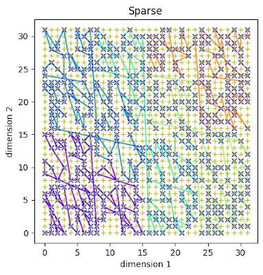
This greater efficiency is true even if we don't take the unlikely case that the data is tightly packed. Below are examples where the data is more realistic and not every possible point (a red +) is actually associated with data (a blue circle).

A Hilbert curve over sparse data

To understand what is going on, we need to appreciate Gray Codes [Wikipedia] which is an alternative numbering system in binary where adjacent numbers only differ by one bit changing (see that parallel with Hilbert curves?). For each bit, for each dimension, we create a mask from the Gray code and do some bit manipulation found here and we'll eventually have a bijective map ℤ^d → ℤ.

The jumps between adjacent data points is less extreme in Hilbert curves. You can see this by-eye if look at a slightly larger space (code here):

A Hilbert curve over sparse data

Typically, the jumps between data points are never more than a couple of positions (average of 1.433). Now, compare this to a similar space using Z-Ordering:

Z-Order over a similar sparse space

and you can see larger jumps between some data points. The average is 2.083 in this run. That's 45% higher than in the Hilbert curve.

Hilbert curves are not currently implemented in Apache Iceberg but are in Databrick's Delta Lake.

GPU vs CPU vs AVX

Vector databases are all the rage. So, I looked at three different ways of multiplying vectors: CPU, GPU and Advanced Vector Extensions that leverages SIMD instructions if your hardware supports them. To access the GPU, I'm using the Tornado Java VM. For AVX, I'm using the JVM's jdk.incubator.vector module, available since JDK16.

(Code in my GitHub repo here).

The reason we're looking at vector mulitplication is that searching for vectors (what the vector DB is all about) usually uses something like the approximate nearest neighbour algorithm. One way to implement it is something like Ethan Lui's implementation mentioned in a past blogpost here. Briefly: it multiplies your vector by random vectors resulting in a vector whose bits are on or off depending on the sign of each element in the product.

The results are as follow (note, the GPU is a Quadro T2000 that apparently has 4gb of memory, 1024 cores and a bandwidth of 128 gigabits per second).

You can see that there is a huge fixed cost to using the GPU but once you get sufficiently large vectors, it's worth it. But what causes this fixed cost?

On my Intel Xeon E-2286M  CPU @ 2.40GHz, kernel calls take typically 17.8ns.

  17.776 ±(99.9%) 0.229 ns/op [Average]

  (min, avg, max) = (17.462, 17.776, 19.040), stdev = 0.306

  CI (99.9%): [17.547, 18.005] (assumes normal distribution)

JNI calls take a little longer at about 21.9ns:

  21.853 ±(99.9%) 0.488 ns/op [Average]

  (min, avg, max) = (21.345, 21.853, 23.254), stdev = 0.651

  CI (99.9%): [21.365, 22.340] (assumes normal distribution)

So, it doesn't seem that the fixed costs incurred in the GPU vector multiplication is due to context switching when calling the kernel or calls via JNI.

Note the maximum vector size for this test was 8 388 608 floats. 

That's 268 435 456 bits or 0.25 gigabits.

Based on just bandwidth alone and ignoring everything else, each call should be about 1.95ms. This matches the average observed time (1.94971ms). 

This suggests the actual calculation is incredibly fast and only the low bandwidth is slowing it down. Tornado VM appears to have minimal room for improvement - you really are getting the best you can out of the hardware.