Spark Numerical Optimization

Neural Net Gradient Optimization

Spark's implementation of artificial neural nets is a little sparse. For instance, the only activation function is the private SigmoidFunction. It seems like there are other ways of training large ANNs at scale. This is an interesting article where data scientists used Deep Java Library (DJL - not to be confused with DL4J) in a Spark framework to orchestrate PyTorch model training.

In theory, one could add one's own activation functions and extract the weights that Spark generated. I took a look at the code of MultiLayerPerceptronClassifier and saw how in each epoch, it broadcasts the weights to all the executors and then uses RDD.treeAggregate to compute the gradient per vector, per partition and then combine them all. In the case of BFGS numerical optimization technique, the Breeze library is used and the call to treeAggregate was invoked as a callback to its BFGS implementation. Note that this was done on Spark's driver and the the loss and averaged gradient are calculated there.

Here, "we cannot write down the actual mathematical formula for the function we’re optimizing. (The technical term for the function that is being optimized is response surface.)" [1]

The format of the broadcast weights confused me at first as they're a one dimensional vector when I was expecting matrices (see Neural Nets are just Matrices). On closer inspection I saw that this vector contained all the values in all the matrices for all the layers and was sliced and diced accordingly.

Hyperparameter Optimization via Randomisation

One level up, a meta-optimization if you like, we want to tune the parameters for the neural nets (choice of activation function, size and cardinality of layers etc). Spark only offers ParamGridBuilder out of the box. This is really just a simple class that creates a Cartesian product of possible parameters. This is fed to CrossValidator.setEstimatorParamMaps as a simple Array so the cross validator can explore a parameter space by brute force.

There is a more clever way that involves a random search. "for any distribution over a sample space with a finite maximum, the maximum of 60 random observations lies within the top 5% of the true maximum, with 95% probability" [1]

It seems odd but it's true. Let's look at the probability of not being in the top 5%. And let's call this top 5% space, X. Then:

P(x ∈ X) = 0.05

so, the probability of a random point not being in the top 5% is:

P(¬x ∈ X) = 1 - 0.05

Now, given N points, the probability of them all not being in the top 5% is:

P(¬x_i ∈ X ∀i) = (1 - 0.05)^N

So, the probability being in the top 5% is one minus this. 

Say, we want 95% probability we're in the top 5%, solve this equation and you'll see N is slightly less than 60. QED.

Exploration of Space

The state space of parameters can be explored for maxima or minima via various techniques. There are more intelligent ways of doing it but one may is using Monte Carlo techniques. Here in my GitHub account is a Python/Theano/PyMC3 example using Metropolis-Hastings to sample from a beautifully named Himmelblau function. This function is nice as we know analytically that it happens to have four local minima. But let's pretend we don't know that:

The Himmelblau function (top) and finding its minima (bottom)

The path to explore the space starts in a random place but quickly finds one of the local minima.

We might be lucky and the algorithm (non-deterministically) jumps out of its local minima and finds another:

Finding two (equal) local minima.

But Metropolis-Hastings generally needs a lot of samples to find all local minima (in the diagram above, it was 30k and we only found two of the four). But it can find at least find some local minimum quite easily in as few as 60 steps:

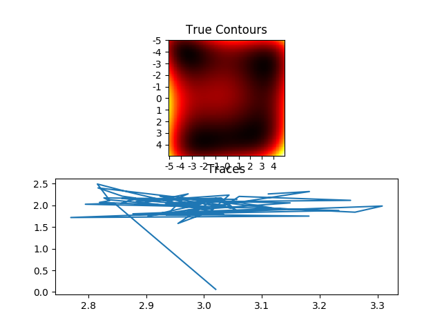
Local minima (3.0, 2.0) found in 60 steps

The MH algorithm adapts with each step whereas the Spark cross validation API expects the parameter co-ordinates to be fed to it a priori. If Spark is to have a more intelligent search space agent, it won't be via this class.

[1] Alice Zheng on O'Reilly

Feature Engineering Time Series

"The loss of information that I mentioned above could actually be a useful feature of the Fourier Transformation. Let me explain. Your timeseries probably has some noise in it. One very useful thing that you can do in your feature engineering process would be to take the Fourier Transformation of your time-series. It will probably look pretty chaotic when you do that, because there is some noise built into the signal. So now that you are in the frequency-domain, you can just threshold your transformed data-set. You can do this by simply setting an arbitrary threshold say any frequency with an amplitude greater than 10, any amplitude less than 10, you set to zero. And then you can transform the series back to the time-domain. What you will find when you do this is that your time-series has been simplified. There is less noise. Essentially, what you have done is you have applied a filter to your data. You have filtered out the components of the signal that are likely noise." - Ryan Barnes

Some Fourier transform examples

With code stolen from here [SO] we can see an example:

"A property of the Fourier Transform which is used, for example, for the removal of additive noise, is its distributivity over addition." [1]

When you look at the code to generate this, you'll see it mention it will try to "remove DC". In this context, DC means the average (that is, frequency 0) values. This is a historical legacy of electrical engineering where DC means the Direct Current rather than the waves that make AC electricity.

Now, let's try a 2D representation where I'm actually trying to simulate human behaviour. Let's say it's people going to Church or Synagogue one day per week. We can do this "because the Fourier Transform is separable ... Using these two formulas, the spatial domain image is first transformed into an intermediate image using N one-dimensional Fourier Transforms. This intermediate image is then transformed into the final image, again using N one-dimensional Fourier Transforms." [1]

Can Fourier transforms pick it out of the data? (Code is on my GitHub repository):

Fig 2: Regular activity. Time is the y-axis in the top graphic. The second is frequency space. The third, amplitudes per column.

The first thing to notice is that instead of our spectrum having a peak both side of the origin for the frequency, there are many peaks at multiples of the frequency. These are the harmonics. The reason Figure 1 does not have them is that the signal is made of two pure sinusoidal waves. There are no other frequencies at play.

Now, let's add some noise.

Regular activity with noise

Our regular periodicity is still the most prominent signal in frequency space and the lowest harmonic does indeed correspond to to a regular event - in this case, it's something that happens every 8 days and the lowest harmonic is indeed at 0.125.

Worked example

So much for the theory, let's examine the practise. I note that my /var/log/syslog has lots of noise in it. I want to de-noise it to see if there is something suspicious in it. I used this code in my GitHub repository to spot irregular activity. Note, this is a very simple implementation that just looks at the process that logged an event and its time. I'll make it more sophisticated later.

Anyway, running the parsed log through a Fourier transform resulted in this:

A Fourier transform of syslog events

We can see that there are clearly some regulars so taking them out, we see that the three (arbitrary number alert) most irregular events came from anacron, systemd and nvidia-persistenced. Looking at these logs in syslog did indeed indicated that they were isolated events albeit nothing to worry about (dockerd and containerd were the most regular naggers).

[1]  University of Edinburgh

Neural Nets and Anomaly Detection pt 1

More playing with anomaly detection, this time with Keras. All the data is synthetic and can be generated from the code on my GitHub here.

The Data

Our data looks like this:

Typical synthetic data

The top row shows noisy data that have a clear global periodicity. The bottow row shows noisy data with each column having a periodicity independent of the other columns.

Can a Variational Auto Encoder tell the difference?

The Model

The code for our neural net was adapted from this StackOverflow answer here. Very quickly (roughly 10 epochs), the VAE was able to differentiate which group a given square was in with an accuracy of about 90%.

The data projected onto the VAE's bottleneck

Note that I am not going to tune the VAE to get the last drop of accuracy. I'm happy with about 90%.

Note that the trick with VAEs is that the data with which we train it is also the data that we expect. This is simply because we're asking the neural net to reproduce what it's been given. It won't be exact at all since we're deliberately compressing the data through a bottleneck. This is the very definition of an auto encoder. The 'variational' term comes from the fact that the neural net learns the probabilities of the distribution representing the data [Quora].

The Results

The trouble with VAEs is that although you might be able to print a pretty graph of the rendered data, you might need some algorithm to differentiate all the data for you. I'm going to use SciKitLearn to run a KMeans algorithm since I know there are exactly 2 groups (that is, k=2 here).

This is fine in this example where I have two groups of 256 elements. What if we're faced with imbalanced data and are looking for outliers? KMeans does not do so well with that. It doggedly tries to find two clusters of roughly equal size giving an accuracy of about 50% - the monkey score.

Spot the outlier

To this end, we can use the DBScan algorithm, again from SKLearn. This finds my outlier but does take a bit of tuning.

Still playing...

Hypothesis Testing Notes

Recipe

A hypothesis test is only a partial answer to the question "am I being fooled by randomness?". It does not address sampling bias nor measurement errors both of which might be responsible for the apparent effect. [1]

The way to put a hypothesis test together is:

1. Define a test statistic.

2. Define a null hypothesis.

3. Ensure the model can generate synthetic data.

4. Calculate the p-value by generating data (step 3) that fulfills the test statistic.

"All hypothesis tests fit into this framework." [2]

p-value

"Ideally we should compute the probability of seeing the effect (E) under both hypotheses; that is P(E | H0) and P(E | HA).  But formulating HA is not always easy, so in conventional hypothesis testing, we just compute P(E | H0), which is the p-value" [3]

Given our recipe above, this is how we'd calculate the p-value of a (potentially) crooked dice.

1. Run 1000 simulations
2. Find the chi-squared value for each
3. Count the number above a threshold defined by the chi-squared value for the (expected, actual) tuple.
4. Divide by the 1000 trials and you have the p-value

Note that "the p-value depends on the choice of test statistic and the model of the null hypothesis, and sometimes these choices determine whether an effect is statistically significant or not." [4] "If different models yield very different results, that's a useful warning that the results are open to interpretation." [2]

Worked Example

Problem: In ThinkStats2, the assertion is made that first babies arrive earlier than subsequent babies. Given pregnancy duration for 4413 first babies and 4735 subsequent births, there is a 0.078 week different between the two means. Is this significant?

Methodology: we repeatedly sample pairs of births and measure their difference. After N samples, we calculate our mean difference.

With the null hypothesis, we assume there is no effect and sample from all data without distinguishing between the two labels. We do this for N iterations by shuffling the original data and assigning each datum to one of two groups. Then, we take the difference in the means of those two groups. After N samples, we calculate our mean difference.

1 Statistical Inference is only mostly wrong - Downey

2 There is still only one test - Downey

3 There is only one test! - Downey

4 Think Stats2 - Downey

Kleislis

What are they?

Accordingly, the functions that we try to compose are actually A => Monad[B] . A wrapper around them, a category that is naturally associated with a Monad[B], is called a Kleisli category. A => Monad[B] or Kleisli arrows is just a way to compose these sort of functions, nothing more... 

Fun fact: If you compose Kleisli arrows for IO monad, you will get a description of your computer program. Your computer program is essentially one gigantic Kleisli arrow, with some input and output of Unit that acts as a description, and a runtime environment that executes this program works as an interpreter.

[Pavel Zaytsev on Medium.com]

Rob Norris @tpolecat Nov 20 20:39

Kleislis compose, the equivalent bare functions don't. It's just a matter of convenience.
Kleisli[F, A, B] and A => F[B] are isomorphic, pick whichever works better.

John D Cook has a blog post here how the use of Kleislis could have saved the Mars lander from failing (TL;DR; the conversion from kilometers to miles was done twice).

Why are they useful?

They compose whereas monads (usually) don't.

If you know how to map over A[X] and over B[X] you also know how to map over A[B[X]]. Automagically. For free. 

This is untrue for Monad: knowing how to flatMap over A[X] and B[X] doesn’t grant you the power of magically deriving a flatMap for A[B[X]]. 

It turns out this is a well known fact: Monads do not compose, at least not generically.

[Blog of Gabriele Petronella]

From Rob Norris' talk, Functional Programming with Effects

[Rob's talk is here].

Using Haskell notation: "there is a way to compose functions like a -> m b and b -> m c into a -> m c (like the function here, from String to Set[String]). They are called Kleisli functions" [SO]

Ryan Peters [@sloshy on Gitter Jul 14 18:21 2020] describes why he likes Kleisli's for Dependency Injection:

damnit I keep stumbling into Kleisli by accident... 

My architecture as of late has looked something like this:

Config object defining how to read in config arguments/env (using Decline or Ciris)

Dependencies case class that has a constructor which depends on that Config and tries to read it in, converting those values to all of my dependencies.

Anything that needs different dependencies, like concurrent jobs or other processes, is defined as a Kleisli as mentioned.

Main loads a single Resource[IO, Dependencies] and converts all of my Kleisli jobs into Kleisli[IO, Dependencies, ExitCode] and runs it at once.

Kleisli is intimately related with "first do X then do Y" (sequencing) [Gavin Bisesi Gitter May 06 21:02, 2020]. Also, note that ReaderT == Kleisli [Adam Rosien Gitter May 06 19:28 2020]

Usage in HTTP4S

[Gabriel Volpe @gvolpe Jul 06 16:17 2020]

So, HttpRoutes is an alias for 

Kleisli[OptionT[F, *], Request[F], Response[F]]

We say 

def handle(routes: HttpRoutes[F]): HttpRoutes[F] = ...

So that's the type we are expecting to have (we are annotating our function [with] the expected type), meaning we don't need to do the same again within the Kleisli block because the types can be inferred. It would be a different story if we wouldn't have told the compiler what the expected type is.

Then we have the implementation:

Kleisli { req =>

      OptionT {

        A.handleErrorWith(routes.run(req).value)(e =>
          A.map(handler(e))(Option(_)))

      }

    }

Kleisli { ... } is the same as calling Kleisli.apply. So [within] this block, we expect the type to be 

Request[F] => OptionT[F, Response[F]]

Remember that req can be inferred by the compiler, so we know we have req: Request[F]

Then again we call OptionT { ... } which is the same as OptionT.apply. So [within] this block, we expect the type to be 

F[Option[Response]].

Now we get to the final block

A.handleErrorWith(routes.run(req).value)(e => 
   A.map(handler(e))(Option(_))
) 

Let's recap on the types we have

routes:  HttpRoutes[F]

req:     Request[F]

handler: E => F[Response[F]]

A:       ApplicativeError[F, Throwable]

A good exercise would be to split every single part to understand what the types are

routes.run(req) effectively runs the Kleisli by feeding a Request[F], which gives us an OptionT[F, Response[F]]. So we call .value on it to get F[Option[Response[F]]

Now here's the type signature of handleErrorWith

def handleErrorWith[A](fa: F[A])(f: E => F[A]): F[A]

fa is F[Option[Response[F]] for us

so the second part should be 

E => F[Option[Response[F]] 

but notice that handler is defined as 

E => F[Response[F]] 

so we perform that final map(Option(_)) to lift that Response[F] into an Option[Response[F]].

A worked example using HTTP4S

I found this sample on GitHub informative. It presents an HTTP server using Http4s, a database from H2 (from a quick sbt 'show dependencyClasspathFiles' or sbt dependencyTree), Quill and even Flyway to update the database schema. All of this in less than 150 lines!

The whole app is basically this line:

  private val httpApp: Kleisli[IO, Request[IO], Response[IO]] = (videos <+> tags <+> videotags).orNotFound 

where videos, tags and videotags are all HttpRoutes which is just an alias as defined above by Gabriel.

But what is this <+> magic? Well, we're combining Kleisli's by treating their content as semigroups. The results seemed a little counter intuitive to me to begin with. Run this code:

  val add1      = Kleisli[List, Int, Int](x => List(x + 1))

  val divide10  = Kleisli[List, Int, Int](x => List(x / 10))

  val add1Div10 = add1 <+> divide10

  println(add1Div10.run(99))

and you'll see:

List(100, 9)

Straight forward so far. The call to Kleisli.run executed both functions on the input and used an implicit semigroup to glue the answers together within the List.

But HttpRoutes does not deal with Lists, it deals with OptionTs - a monad transformer for Options. How they behave is demonstrated in my GitHub project. Basically, the binary operator defers to OptionTSemigroupK and it looks like this:

def combineK[A](x: OptionT[F, A], y: OptionT[F, A]): OptionT[F, A] = x.orElse(y)

For example, if our F was a List[Int] (that is, we're gluing together OptionT[List, Int]s) then calling <+> on them will result in a Kleisli whose value is a list with just the first Some (or a single None if they're both Nones). 

Note that if our F were IO then the effect associated with any but the first OptionT would not be run (as demonstrated here in my GitHub). In our HTTP app, the flow short circuits on the first combined function that gives a satisfactory answer.

But now we're getting away from Kleisi's and into semigroups. Suffice to say, composing the Kleisli will glue the results together according to the laws of their semigroup.

Bootstrapping

When trying to evaluate which method most increases the accuracy of a neural net, I had previously used a Bayesian method. But, with a technique known as bootstrapping, I could calculate the confidence interval using classical methods.

"The bootstrap is a method for estimating standard errors and computing confidence intervals" [1]. It's very useful when you have small amounts of data. Using it, we resample (with replacement) the original data many, many times until a histogram of our results is more informative.

"It must be noted that increasing the number of resamples, m, will not increase the amount of information in the data. That is, resampling the original set 100,000 times is not more useful than only resampling it 1,000 times. The amount of information within the set is dependent on the sample size, n, which will remain constant throughout each resample. The benefit of more resamples, then, is to derive a better estimate of the sampling distribution." [TowardsDataScience]

Recall that I only had 9 data points for my two methods (L1 and L2 normalisation of the data). But using the bootstrap technique, this lumpy data could be transformed like this for L1 normalization:

Bootstrapped
accuracy using L1 normalization

and this for L2  normalization:

Bootstrapped 
accuracy using L2 normalization

Note how a sparse distribution becomes much more informative.

By excluding the lowest 5% and the highest 5% of results from bootstrapping we can calculate the confidence interval such:

• the 90% confidence interval for L1 normalization was [0.9466, 0.9504].
• the 90% confidence interval for L2 normalization was [0.9412, 0.9456].

[Python code lives in my GitHub]

Note some caveats with confidence intervals:

"... a 95% confidence interval does not indicate that the parameter of interest has a 95% probability of being within the interval.  Ironically, the situation is worse when the sample size is large.  In that case, the CI is usually small, other sources of error dominate, and the CI is less likely to contain the actual value." Statistical Inference is only mostly wrong - Downey

Also note that boostrapping depends on the Central Limit Theorem - the idea that sampling the mean of most distributions eventually forms a Gaussian. This is not universally true. For instance, the Cauchy distribution is of the form (1+x²)^-1 which you might recognise as a standard integral that can be integrated from -∞ to ∞ (giving a function dependent on arctan) so it can be a valid probability distribution. However, if we tried to find the mean by integrating x/(1+x²) (try using integration by substitution and note that it is symmetric around the y-axis) we get an infinity. Hmm.

Indeed, if we change the Python code to generate data from a Cauchy so:

from scipy.stats import cauchy
...
    data = cauchy.rvs(size=n) 

then don't be surprised if you see something like this:

Bootstrapping a Cauchy

Which is not very useful at all.

[1] "All of Statistics" Wasserman.

Notes on Comonads

This excellent post by Eli Jordan can be summarized as comonads offer counit and cojoin, the opposites of on unit and join (or flatten as Cats calls it) monads. 

Why this is useful is that it can model a use case where there is the notion of focus. To demonstrate this, Jordan has created an implementation of Conway's Game of Life (code). Here, the focus is a cell which we determine is either on or off given its neighbours. (Another example of how comonads use focus can be found here where we traverse a graph, node by node).

The case class on which we will call counit and cojoin is an abstraction, Store[S, A], but for the Game of Life example, it is the grid on which the changing cells live. Notably, Store is instantiated with two arguments, 

1. lookup: S => A
2. index: S  

Specifically for our game, these represent:

1. a mapping from a co-ordinate (S) to a Boolean (A) representing whether the corresponding cell is turned on or off.
2. the co-ordinates of the cell that has the focus. That is, S for us is of type (Int, Int).

For each step in our game, we ask our grid (Store) what the neighbourhood is like (lookup) for its focused cell (index). 

We do this by calling its Cats coflatMap function (that we added via a type class) that takes a grid and returns a Boolean. 

This is where it gets interesting. You'll notice that Store has the potential for a partially applied constructor. That is, it looks like:

case class Store[S, A](lookup: S => A)(val index: S) { ...

So, if we instantiate Store with just a S => A, we actually have a S => Store[S, A].

In our Game of Life, this means that for the coflatMap branch of the code, the grid is not actually a mapping to whether the cell is turned on or off (F[Boolean]) but to the grid of the previous iteration on which we will apply Conway's rules to derive Boolean on/off  mappings. That is, it's our cojoin of type of F[F[Boolean]] that needs to be flattened.

Memoization

Recalculating Conway's rules recursively is expensive. Without memoization, you'll see deep stacks. Using jconsole, I saw quite a few:

- eliminated <owner is scalar replaced> (a Store) at Store.counit(Life.scala:69)

which apparently "represents a redundant lock that has been removed in the bytecode." [SO]. This is because the code on each lookup is trying to recalculate the grid from scatch. Memoization prevents this by caching the grid of the last iteration.

What triggers this recalculation is the rendering of the 20x20 grid. This grid obviously leads to 400 evaluations. But the grid (Store) of each iteration has a reference its predecessor's 400 on which it must calculate Conway's rules. Not only do we not want to recalculate that grid from the game's beginning, we don't want to perform a further 3600 (=400 * 8 neighbours) calculation for cells we've already evaluated - hence the caching.