![]() |
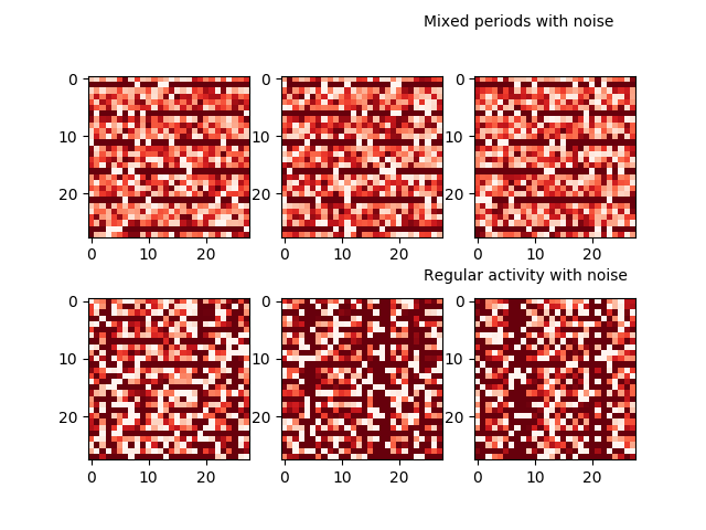
| Typical synthetic data |
![]() |
| The data projected onto the VAE's bottleneck |
![]() |
| Spot the outlier |
Musings on Data Science, Software Architecture, Functional Programming and whatnot.
![]() |
| Typical synthetic data |
![]() |
| The data projected onto the VAE's bottleneck |
![]() |
| Spot the outlier |
Recipe
Accordingly, the functions that we try to compose are actually A => Monad[B] . A wrapper around them, a category that is naturally associated with a Monad[B], is called a Kleisli category. A => Monad[B] or Kleisli arrows is just a way to compose these sort of functions, nothing more...
Fun fact: If you compose Kleisli arrows for IO monad, you will get a description of your computer program. Your computer program is essentially one gigantic Kleisli arrow, with some input and output of Unit that acts as a description, and a runtime environment that executes this program works as an interpreter.[Pavel Zaytsev on Medium.com]
Kleislis compose, the equivalent bare functions don't. It's just a matter of convenience.
Kleisli[F, A, B] and A => F[B] are isomorphic, pick whichever works better.
If you know how to map over A[X] and over B[X] you also know how to map over A[B[X]]. Automagically. For free.
This is untrue for Monad: knowing how to flatMap over A[X] and B[X] doesn’t grant you the power of magically deriving a flatMap for A[B[X]].
It turns out this is a well known fact: Monads do not compose, at least not generically.[Blog of Gabriele Petronella]
![]() |
| From Rob Norris' talk, Functional Programming with Effects |
damnit I keep stumbling into Kleisli by accident...
My architecture as of late has looked something like this:Config object defining how to read in config arguments/env (using Decline or Ciris)Dependencies case class that has a constructor which depends on that Config and tries to read it in, converting those values to all of my dependencies.Anything that needs different dependencies, like concurrent jobs or other processes, is defined as a Kleisli as mentioned.Main loads a single Resource[IO, Dependencies] and converts all of my Kleisli jobs into Kleisli[IO, Dependencies, ExitCode] and runs it at once.
So, HttpRoutes is an alias forKleisli[OptionT[F, *], Request[F], Response[F]]We saydef handle(routes: HttpRoutes[F]): HttpRoutes[F] = ...So that's the type we are expecting to have (we are annotating our function [with] the expected type), meaning we don't need to do the same again within the Kleisli block because the types can be inferred. It would be a different story if we wouldn't have told the compiler what the expected type is.Then we have the implementation:Kleisli { req =>OptionT {A.handleErrorWith(routes.run(req).value)(e =>
A.map(handler(e))(Option(_)))}}Kleisli { ... } is the same as calling Kleisli.apply. So [within] this block, we expect the type to be
Request[F] => OptionT[F, Response[F]]Remember that req can be inferred by the compiler, so we know we have req: Request[F]Then again we call OptionT { ... } which is the same as OptionT.apply. So [within] this block, we expect the type to be
F[Option[Response]].Now we get to the final blockA.handleErrorWith(routes.run(req).value)(e =>
A.map(handler(e))(Option(_))
)
Let's recap on the types we haveroutes: HttpRoutes[F]req: Request[F]handler: E => F[Response[F]]A: ApplicativeError[F, Throwable]A good exercise would be to split every single part to understand what the types areroutes.run(req) effectively runs the Kleisli by feeding a Request[F], which gives us an OptionT[F, Response[F]]. So we call .value on it to get F[Option[Response[F]]Now here's the type signature of handleErrorWithdef handleErrorWith[A](fa: F[A])(f: E => F[A]): F[A]fa is F[Option[Response[F]] for usso the second part should beE => F[Option[Response[F]]but notice that handler is defined asE => F[Response[F]]so we perform that final map(Option(_)) to lift that Response[F] into an Option[Response[F]].
When trying to evaluate which method most increases the accuracy of a neural net, I had previously used a Bayesian method. But, with a technique known as bootstrapping, I could calculate the confidence interval using classical methods.
"The bootstrap is a method for estimating standard errors and computing confidence intervals" [1]. It's very useful when you have small amounts of data. Using it, we resample (with replacement) the original data many, many times until a histogram of our results is more informative.
"It must be noted that increasing the number of resamples, m, will not increase the amount of information in the data. That is, resampling the original set 100,000 times is not more useful than only resampling it 1,000 times. The amount of information within the set is dependent on the sample size, n, which will remain constant throughout each resample. The benefit of more resamples, then, is to derive a better estimate of the sampling distribution." [TowardsDataScience]
Recall that I only had 9 data points for my two methods (L1 and L2 normalisation of the data). But using the bootstrap technique, this lumpy data could be transformed like this for L1 normalization:
![]() |
| Bootstrapped accuracy using L1 normalization |
and this for L2 normalization:
![]() |
| Bootstrapped accuracy using L2 normalization |
[Python code lives in my GitHub]
Note some caveats with confidence intervals:
"... a 95% confidence interval does not indicate that the parameter of interest has a 95% probability of being within the interval. Ironically, the situation is worse when the sample size is large. In that case, the CI is usually small, other sources of error dominate, and the CI is less likely to contain the actual value." Statistical Inference is only mostly wrong - Downey
Also note that boostrapping depends on the Central Limit Theorem - the idea that sampling the mean of most distributions eventually forms a Gaussian. This is not universally true. For instance, the Cauchy distribution is of the form (1+x2)-1 which you might recognise as a standard integral that can be integrated from -∞ to ∞ (giving a function dependent on arctan) so it can be a valid probability distribution. However, if we tried to find the mean by integrating x/(1+x2) (try using integration by substitution and note that it is symmetric around the y-axis) we get an infinity. Hmm.
Indeed, if we change the Python code to generate data from a Cauchy so:
from scipy.stats import cauchy
...
data = cauchy.rvs(size=n)
then don't be surprised if you see something like this:
| Bootstrapping a Cauchy |
Which is not very useful at all.
[1] "All of Statistics" Wasserman.
This excellent post by Eli Jordan can be summarized as comonads offer counit and cojoin, the opposites of on unit and join (or flatten as Cats calls it) monads.
Why this is useful is that it can model a use case where there is the notion of focus. To demonstrate this, Jordan has created an implementation of Conway's Game of Life (code). Here, the focus is a cell which we determine is either on or off given its neighbours. (Another example of how comonads use focus can be found here where we traverse a graph, node by node).
The case class on which we will call counit and cojoin is an abstraction, Store[S, A], but for the Game of Life example, it is the grid on which the changing cells live. Notably, Store is instantiated with two arguments,
Specifically for our game, these represent:
For each step in our game, we ask our grid (Store) what the neighbourhood is like (lookup) for its focused cell (index).
We do this by calling its Cats coflatMap function (that we added via a type class) that takes a grid and returns a Boolean.
This is where it gets interesting. You'll notice that Store has the potential for a partially applied constructor. That is, it looks like:
case class Store[S, A](lookup: S => A)(val index: S) { ...
So, if we instantiate Store with just a S => A, we actually have a S => Store[S, A].
In our Game of Life, this means that for the coflatMap branch of the code, the grid is not actually a mapping to whether the cell is turned on or off (F[Boolean]) but to the grid of the previous iteration on which we will apply Conway's rules to derive Boolean on/off mappings. That is, it's our cojoin of type of F[F[Boolean]] that needs to be flattened.
Memoization
Recalculating Conway's rules recursively is expensive. Without memoization, you'll see deep stacks. Using jconsole, I saw quite a few:
- eliminated <owner is scalar replaced> (a Store) at Store.counit(Life.scala:69)
In our topology, we have a Databricks Spark Structured Streaming job reading from an HDInsights Kafka cluster that is VNet injected into our subscription. So, disaster recovery has to take into account two things:
This Microsoft document outlines the usual way in securing your data in Kafka (high replication factors for disk writes; high insync replicas for in-memory writes; high acknowledgement factor etc). In addition, an HDInsight cluster are backed by managed disks that provide "three replicas of your data" each witihin their own availability zone that's "equipped with independent power, cooling, and networking" [Azure docs].
So, within a region, things look peachy. Now, how do we get these Kafka messages replicating across region? The HDInisghts documentation suggests using Apache MirrorMaker but note one critical thing it says:
"Mirroring should not be considered as a means to achieve fault-tolerance. The offset to items within a topic are different between the primary and secondary clusters, so clients cannot use the two interchangeably."
This is worrying. Indeed, there is a KIP to make MirrorMaker 2 fix this problem and others like it (like differences in partitions within topics of the same name; messages entering infinite loops etc). Confluent is pushing its Replicator that (it claims) is a more complete solution (there's a Docker trial for it here). And, there is Brooklin, but Azure says this would be self-managed.
Spark and Blobs
At the moment, all the data goes into one region. The business is aware that in the event of, say, a terrorist attack of the data centres, data will be lost. But even the infrastructure guys have the data being replicated from one region to another, note this caveat in the Azure documentation (emphasis mine):
"Because data is written asynchronously from the primary region to the secondary region, there is always a delay before a write to the primary region is copied to the secondary region. If the primary region becomes unavailable, the most recent writes may not yet have been copied to the secondary region."
But let's say that nothing so dramatic happens. Let's assume our data is there once we get our region back on its feet. In the meantime, what has been landed by SSS in the backup region is incompatible with what came before. This is because Spark stores its Kafka offsets in a folder in Gen2. It's just as well Spark is not writing to the directory that the erstwhile live region was using. If we had been writing to a directory that was common to both regions, some finagling would have to be done as we points the Spark job at another directory, effecting the RTO if not RPO.
Aside: A disaster of a different kind
In the old days of on-prem Hadoop clusters, you might see a problem where too many files were created. The consequence would be the Name Node goes down. Sometimes deciphering the Azure documentation is hard but this link says the "Maximum number of blob containers, blobs, file shares, tables, queues, entities, or messages per storage account" has "No limit".
Hopefully (caveat: I have not tested this in the wild) this problem has gone away.
Continuing the investigation into a lack of cache coherency in Databricks in my previous post, I've raised the issue with the people at Azure.
In the document a representative from Microsoft pointed me to, there are two caches at play: Delta Cache and Apache Spark cache. "The Delta cache accelerates data reads by creating copies of remote files in nodes’ local storage" and is enabled by default on certain clusters. In effect, you get it for free when you use Databricks
The Apache Spark cache is familiar one that is invoked by calling Dataset.cache().
My first complaint is that these two caches behave inconsistently. In the Delta Cache, updates are immediately available. But if we use the Apache Spark cache in conjunction with the Databrick's Delta Lake (not to be confused with the orthogonal Delta Cache), the data is frozen in time.
Now, in the Spark world, Datasets are strictly immutable. But Delta Lake "provides ACID transactions ... on top of your existing data lake and is fully compatible with Apache Spark APIs." Well, once I've invoked .cache(), and update the Delta Lake in the standard way:
df.write
.format("delta")
.mode("overwrite")
.option("replaceWhere", CONDITION_STRING)
.save(HDFS_DIRECTORY)
What is, perhaps, even more bizarre can be seen when I try to read the data afresh. A second, totally independent call (but using the same Spark session) to read the data like this:
session.read.format("delta").load(dir)
This brings me to my next complaint - the leaky abstraction. Databricks is trying to retrofit ACID transactions on an API that was built with immutability at its core. The claim that it's "fully compatible with Apache Spark APIs" seems not enitrely true.
I have a meeting scheduled with the MS representative who is currently of the opinion that we should just never call .cache(). On Azure Databrics, this does not seem too bad as the Delta Cache seems pretty fast. It sucks for anybody using Delta Lake on just HDFS.
Summary
If you call .cache() on a Spark Dataset while using Databricks Delta Lake format you will not be able to: