Methods that may or may not compile in Scala

If you want to sum some integers in a List, you just call the sum method. So far, so obvious. But if the list does not hold elements that are summable, how does Scala give you a method that you may or may not call?

The sum method lives in TraversableOnce and the signature looks like this:

  def sum[B >: A](implicit num: Numeric[B]): B = ...

Here [B >: A] says B must be a superclass of A, the type of elements in the list. The implicit says there must exist in the ether something that provides the functionality in trait Numeric for type B (the functionality for plus, minus etc).

Now, for Int, Double etc you get these for free in the Numeric object that's standard to Scala where you see, for example:

  trait IntIsIntegral extends Integral[Int] { ...

which is pulled into the implicit ether with:

  implicit object IntIsIntegral extends IntIsIntegral with Ordering.IntOrdering

in the same file. Note, that unlike Java, Scala's numerics do not extend a common superclass like java.lang.Number.

So, we could happily create our own arithmetic with something like:

  class MyInteger

  trait MyIntegerOrdering extends Ordering[MyInteger] {

    def compare(x: MyInteger, y: MyInteger) = ???

  }

  trait MyIntegral extends Numeric[MyInteger] { // or Integral that extends Numeric[T]

    def plus(x: MyInteger, y: MyInteger): MyInteger = new MyInteger

.

.

.

  }

  implicit object MyIntegerIsIntegral extends MyIntegral with MyIntegerOrdering

It's not a terribly useful arithmetic but it would allow us to have a list of MyIntegers and call sum on it.

Notes on the Future (part 1)

Scala's Futures are very different to Java's. Where Java's Futures encourage blocking by their API, Scala's encourages asynchronous coding... apart from one gotcha that follows shortly.

Futures are Monads so they have all that Monad goodness and we can use them in for comprehensions. Unfortunately, this very idiom can introduce a bug. Take this code:

for {
  i <- Future(5)
  j <- Future(11)
} yield j

It creates two futures operating that return the values 5 and 11, possibly on different threads, and returns a Future that contains 11 just like a good Monad should.

"Here, the beauty of the for comprehension sugar can work against us. The for comprehension hides all of that ugly nesting from us, making it look like these are on the same level, but nesting is indeed happening here. What might look concurrent isn't." [1]

Gotcha

What happens here is the first Future is executed and only then is the second. The solution is simple. The code should look like this:

val iFuture = Future(5)
val jFuture = Future(11)
for {
  i <- iFuture
  j <- jFuture
} yield j

For just returning a number, you probably won't notice anything amiss. But for something more ambitious, you may very well notice that the first cut of this code is sub-optimal.

"Only men's minds could have unmapped into abstraction..."

In Scala, we can get our dirty little hands on the contents of a Future by mapping like:

import scala.concurrent.ExecutionContext

    implicit val xc = ExecutionContext.global // needed for next map:

    j map { value =>
      println("j = " + value)
    }

but there are other ways, too. Being monads, we can flatMap and so if we slightly modify the code in [1]:

  implicit val xc = ExecutionContext.global

  val timeToWait = Duration(5, TimeUnit.SECONDS)

  val future1 = Future[Int] {
    (1 to 3).foldLeft(0) { (a, i) =>
      log("future1 "  + i)
      pause()
      a + i
    }
  }

  val future2 = Future[String] {
    ('A' to 'C').foldLeft("") { (a, c) =>
      log("future2 " + c)
      pause()
      a + c
    }
  }

  def spliceFutures(): Unit = {
    val awaitable = future1 flatMap { numsum: Int =>
      log("in future1.flatMap") // ForkJoinPool-1-worker-1: in future1.flatMap

      future2 map { str: String =>
        log("in future2.map") // ForkJoinPool-1-worker-5: in future2.map
        (numsum, str)
      }
    }

    val awaited = Await.result(awaitable, timeToWait)
    println(awaited) // (6,ABC)
  }

  def log(msg: String): Unit = {
    println(Thread.currentThread().getName() + ": " + msg)
  }

"The most powerful way to use these combinators is in combining the results from futures that are already executing. This means that we can still have a lot of independent futures running, and have another piece of code combine the eventual results from those futures into another "final" future that operates on those results."[1]

You'll notice from the log statements that the code in the map and flatMap run in different threads.

But wait, there's more. You can add callbacks with onSuccess, onFailure and onComplete, all of which have return type of Unit (so you know that the functions passed to it must have side-effects) and there is no guarantee that they'll run on the same thread that ran the body of the Future.

  val onCompleteFn: Try[Boolean] => Unit = {

    case Success(x)   => println(" success: " + x)

    case Failure(err) => println(" failure: " + err + ", " + err.getCause)

  }

.

.

    aFuture onComplete onCompleteFn 

In fact, Future.onComplete is the daddy. All the other combinator methods (map, flatMap, recover, transform etc) all call it. We'll come back to these other combinators in another post.

Problems in your Future

If an Exception is thrown in your Future, then it will be captured in the failure case in onCompleteFn above. But if an Error is thrown, you'll get a Boxed Error.

Another surprise comes from filter. For Lists, Trys and Options, things are quite straightforward:

    val myList = List(1,2,3)
    val filteredList = myList.filter(_ > 10)
    println(filteredList)   // List()

    val myOption = Option(1)
    val filteredOption = myOption.filter(_ > 10)
    println(filteredOption) // None

    val myTry = Try(1)
    val filteredTry = myTry.filter(_ > 10)
    println(filteredTry)    // Failure(java.util.NoSuchElementException: Predicate does not hold for 1)

That is, a filter whose predicate leads to nothing is represented by the "negative" subclass of the monads. However, there is no such class for an "empty" Future.

    import scala.concurrent.ExecutionContext.Implicits._

    import scala.concurrent.duration._

    val myFuture       = Future { 1 }

    val filteredFuture = myFuture filter {_ > 10}

    filteredFuture onComplete {

      case Success(x) => println(s"success: $x")

      case Failure(x) => println(s"failure: $x")

    } // failure: java.util.NoSuchElementException: Future.filter predicate is not satisfied

    Await.result(filteredFuture, 1.second) // Exception in thread "main" java.util.NoSuchElementException: Future.filter predicate is not satisfied

That is, the Failure case is the path taken by onComplete. If we were so foolish to block using Await, then an Exception is thrown.

[1] Akka Concurrency, Derek Wyatt.

Spark Shuffle

... is something you should avoid.  "All shuffle data must be written to disk and then transferred over the network" (from here). This can be very expensive on a large data set. If the data is evenly distributed but a query asks for it to be grouped according to an arbitrary criteria, much movement will ensue. Therefore, groupByKey should be avoided if possible as the ScalaDocs indicate this can be an expensive operation.

However, reduceByKey is much more efficient as it will "perform the merging locally on each mapper before sending results to a reducer" resulting in a much smaller transfer of data between nodes.

So, when we were writing a risk engine with Spark holding all our user-defined Record objects, our code would look something like:

def totalByKey(data: RDD[Record]): RDD[(String, Double)] = {
  data.map(record => record.key -> record.value).reduceByKey(_ + _)
}

which would first turn our Records into key/value pairs then add up all the values for each key without transferring large amounts of data over the network. It avoids this by adding all the values for Records on each node before adding all these subtotals. Only the addition of subtotals requires a network call.

Interestingly, Spark can then do an outer join like this:

val subtotalForDate1 = totalByKey(dataForDate1)

val subtotalForDate2 = totalByKey(dataForDate2)

val outerJoing       = subtotalForDate1.fullOuterJoin(subtotalForDate2)

which returns an RDD of tuples containing the key, the left and the right value. Using this join, we can compare our risk profile from one date to the next.

Note that both reduceByKey and fullOuterJoin don't actually live in the RDD class but the PairRDDFunctions class. They appear to be part of the RDD class by the magic of implicits when the RDD in question contains tuples of pairs.

One last thing to remember is that if you're trying to be clever and reduce collections of elements, you're no better off than using groupByKey. The function reduceByKey is only useful if you are reducing something like a number. If you look at the code for groupByKey you'll see that it's basically doing just that: reducing collections.

Further Reading

Nice article on memory usage.

Try Monads

Martin Odersky in the Reactive Programming course mentions that Try types are not true monads as they violate the Left Unit rule. But if you try (no pun intended) it, Try does indeed appear to obey the rules for monads.

Just to recap, here are the monad rules expressed in Scala:

  def testMonadicPropertiesOfTry[T, U](f: T => Try[U], g: U => Try[U], m: Try[T], x: T, unit: T => Try[T]): Boolean = {

    // Associativity: (m flatMap f) flatMap g == m flatMap (x => f(x) flatMap g)
    def associativity: Boolean = {
      val associativityLhs = (m flatMap f) flatMap g
      val associativityRhs = m flatMap (x => f(x) flatMap g)
      assertEqual(associativityLhs, associativityRhs)
    }
    val associativityResult = Try(associativity)

    // Left unit: unit(x) flatMap f == f(x)
    def leftUnit: Boolean = {
      val leftUnitLhs = unit(x) flatMap f
      val leftUnitRhs = f(x) 
      assertEqual(leftUnitLhs, leftUnitRhs)
    }
    val leftUnitResult = Try(leftUnit)

    // Right unit: m flatMap unit == m
    def rightUnit: Boolean = {
      val rightUnitLhs = m flatMap unit
      assertEqual(rightUnitLhs, m)
    }
    val rightUnitResult = Try(rightUnit)

    (associativityResult, leftUnitResult, rightUnitResult) match {
      case (Success(_), Success(_), Success(_)) => true
      case _ => false
    }
  }

Where my assertEqual method looks like:

  def assertEqual[T](try1: Try[T], try2: Try[T]): Boolean = {
    try1 match {
      case Success(v1) => try2 match {
        case Success(v2) => v1 == v2
        case _ => false
      }
      case Failure(x1) => try2 match {
        case Failure(x2) => x1.toString == x2.toString
        case _ => false
      }
    }
  }

That is, it will compare Failures by looking at the text of their messages. This is because Java exceptions don't have an equals() method.

Now, if we run the code below (borrowed liberally from here) where we're deliberately trying to cause a java.lang.NumberFormatException as the code attempts to convert our 'a' into a numeric:

    def factory[T](x: => T): Try[T] = Try(x)

    def unit[T](x: T): Try[T]   = factory(x)
    def f(x: String): Try[Int]  = factory(x.toInt)
    def g(x: Int): Try[Int]     = factory(x + 1)
    val x                       = "a"
    val m                       = factory(x)

    val isMonadic = testMonadicPropertiesOfTry(f, g, m, x, unit[String])
    println("is monadic? " + isMonadic)

the output says it's true, Try[T] obeys the rules for a monad. What gives?

Mauricio Linhares says: "there is some debate as to if Try[U] is a full monad or not. The problem is that if you think unit(x) is Success(x), then exceptions would be raised when you try to execute the left unit law since flatMap will correctly wrap an exception but the f(x) might not be able to do it. Still, if you assume that the correct unit is Try.apply then this would not be an issue."

So, let's take the first line of the last code snippet and make it thus:

    def factory[T](x: => T): Try[T] = Success(x)

whereupon we are told that Success is not a monad at all. Further investigation reveals that in the leftUnit method:

      val leftUnitLhs = unit(x) flatMap f

works fine but:

      val leftUnitRhs = f(x) 

blows up. The left hand side does not equal the right.

The reason for this is that Success.flatMap catches any NonFatal exceptions just like the constructor of Try. But the constructor of Success does not. And it's this asymmetry that means Try acts like a monad and Success does not.

Further reading

An interesting debate about monads and exceptions here.

The Mathematics of Linear Regression

There's an excellent and free book online called The Elements of Statistical Learning that can be found here. I was browsing through it but hit one of those points where a derivation misses some steps and confuses the reader. It took me a few hours to work it out and it's not too hard but just in case somebody it's the same problem, here is a step-by-step derivation.

The section was on Linear Models and Least Squares (2.3.1) that says:

Ŷ = β̂0 +

p  ∑ j = 1

Xj β̂j

Where β̂₀ is a constant called the bias, β̂ is a vector of coefficients, X is a vector of inputs and Ŷ is the prediction.

To make things more mathematically convenient, let's subsume β̂₀ and the β̂ vector of coefficients into one big vector such that the above equation becomes:

Ŷ = X^Tβ̂

This is exactly the same equation in matrix notation rather than summation notation (X^T is simply the transpose of X).

So, the question becomes what's the optimal value of β̂ ?

Let's re-express this thus: say that we have N trials each with a result y_i (this y has nothing to do with Ŷ). All these results can be put in a vector, y. Let's say the matrix X has N rows each representing p data points that are properties of the system (that is, it's an N x p matrix).

Then the error can be expressed as:

y - X ß

(that is, the output values minus all of the input values that are multiplied by our coefficients). This is what we want to minimize.

How do we do this? Well an obvious way is to find the smallest sum of squares of the differences. So, let's square it:

(y - X ß)^T (y - X ß)

then expand it noting that matrices are distributive, associative but not commutative and:

(A + B)^T = A^T + B^T              (1)

and

(AB)^T = B^T A^T                   (2)

so:

= (y^T - ß^T X^T ) (y - X ß)
= y^Ty - y^T X ß - ß^T X^T y + ß^T X^T X ß

and differentiate it with respect to ß. Where the result of this differentation equals 0 is our optimal value for ß.

The first term is easy to differentiate. There is no dependence of y on ß so it disappears and our equation becomes.

 δ (- y^T X ß - ß^T X^T y + ß^T X^T X ß) = 0     (3)
δß

The next bit is tricky. To help, let's take a look at this useful summary on matrix calculus. The interesting sections for us are Proposition 7 (equations 36 and 37) and Proposition 9 (equation 49). They say:

If:

α = y^T A x

then:

δα = y^T A              (4)
δx

and:

δα = x^T A^T             (5)
δy

where A is independent of and y.

And if:

α = x^T A x

then

δα = 2 x^T A            (6)
δx

where A is symmetric.

Now, take the first term of (3). That's basically equation (4) if we replace A for X and x for ß.

Take the second term of (3). That's basically equation (5) if we replace A for X^T and y for ß and x for y.

Finally, take the third term of (3) and that looks like (6) if we replace A for X^T X and x for ß. How do we know that X^T X is symmetric? Well any matrix multiplied by its transpose is symmetric (see here for the simple proof).

So, taking these three observations, equation (3) becomes:

0 = - y^T X - y^T X + 2 ß^T X^T X
  = 2 ß^T X^T X - 2 y^T X 
  = (ß^T X^T - y^T) X 

Now take the transpose of both sides (the transpose of 0 is 0) and using (1) and (2):

0 = X^T (ß^T X^T - y^T)^T
  = X^T ((ß^T X^T)^T- (y^T)^T)
  = X^T (X ß - y)
  = X^T X ß - X^T y

Rearranging:

X^T X ß = X^T y

and multiplying both sides with (X^T X)^-1 gives:

ß = (X^T X)^-1 X^T y

which is equation 2.6 in The Elements of Statistical Learning. 

K-Means Clustering

K-Means is a clustering algorithm that tells you were the centres are in a set of data points. It "has the major disadvantage that you must pick k [the number of centres] in advance. On the plus side, it’s easy to implement". A simple implementation is just a few lines of Scala although it can be used on a much larger scale in MLLib/Spark.

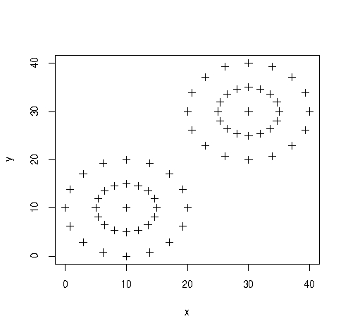
First, let's create some data - just rows of x,y such that when plotted in R it looks like this:

data <- read.csv("/tmp/point.csv", header=F)

matplot(data[,1],data[,2] ,type="p", pch=3, xlab="x", ylab="y")

It's clear where to the human eye that there are 2 clusters here and where their centres are, although it would be much harder just given the raw data.

The snippet of Scala code to calculate K-Means looks something like this:

import scala.collection.immutable.Seq

.

.

case class Distance(point: Point2D, distance: Double)

case class Point2D(x: Double, y: Double)

.

.

  implicit val pointOrdering = new Ordering[Distance] {

    override def compare(x: Distance, y: Distance): Int = (x.distance - y.distance).toInt

  }

  def iterate(centres: Seq[Point2D], others: Seq[Point2D]): Seq[Point2D] = {

    val clusterPairs = centres.map(centre => (centre, Seq[Point2D]()))

    val clusters     = Map(clusterPairs: _*) 

    val assigned     = assign(others, centres, clusters)

    assigned.map(centrePoint => update(centrePoint._2 :+ centrePoint._1)).toSeq.to[collection.immutable.Seq]

  }

  

  def update(points: Seq[Point2D]): Point2D = {

    val distances = points.map(point => sumOfDistances(point, points))

    distances.min.point

  }

  

  def sumOfDistances(point: Point2D, others: Seq[Point2D]): Distance = {

    val distances = others.map(other => distanceFn(other, point))

    Distance(point, distances.sum)

  }

  

  def distancesFrom(centre: Point2D, others: Seq[Point2D]): Seq[Distance] = 

    others.map(point => Distance(point, distanceFn(centre, point)))

Where we call iterate an arbitrary number of times until we're happy we have the centres. The iterate method is initially called with k randomly chosen points that will act as our initial guesses at where the centres are. With each iteration, out guess will be refined.

For each iteration, we do two things. First we assign each point to one of our k estimated centres. Then, within each grouping, we find the point that is the most central. These points will be the basis for our next iteration.

We define the central points within a grouping as those that have the minimum value of adding up all the distances to the other points.

The interesting thing is that the resulting cluster points may change somewhat between runs as the initial choice of points may make a difference. (that is, it's unstable) Therefore, it might be necessary to run it a few times and see the most common outcome.

We can verify the results in R with:

> kmeans(data, 2) # 2 being the number of clusters we're expecting

K-means clustering with 2 clusters of sizes 33, 33

Cluster means:

  V1 V2

1 30 30

2 10 10

Which is the same result as my code when run with 10 iterations and taking the most popular results from 10 runs.

Shapeless

There's a very interesting Scala library called Shapeless that let's you do some weird things with types. One such "what magic is this?!" moment is asserting a checksum derived from a list of numbers is a certain value at compile time rather than run time.

This impressed me no end, even if I can't think of a practical use for it. I'm still trying to get my head around Travis Brown's excellent tutorial since he is so much more clever than me. But here are some notes I made along the way.

First, we borrow a bit from the Peano Axioms where every natural number is a successor to the previous except 0 which has no successor. We model this much like Shapeless does with something like:

  trait NaturalNumber

  trait NaturalNumber0 extends NaturalNumber

  trait NaturalNumberSucceeds[T <: NaturalNumber] extends NaturalNumber

Next we'll have a type representing each and every number. I'll only bother with the natural numbers 0 to 4 to make things simple:

    type Type0 = NaturalNumber0

    type Type1 = NaturalNumberSucceeds[Type0]

    type Type2 = NaturalNumberSucceeds[Type1]

    type Type3 = NaturalNumberSucceeds[Type2]

    type Type4 = NaturalNumberSucceeds[Type3]

This is just shorthand. Really, Type4 is of type:

NaturalNumberSucceeds[NaturalNumberSucceeds[NaturalNumberSucceeds[NaturalNumberSucceeds[NaturalNumber0]]]]

But that's far too verbose.

So much for the types, let's have some instances:

    implicit val _0 = new Type0 {}

    implicit val _1 = new Type1 {}

    implicit val _2 = new Type2 {}

    implicit val _3 = new Type3 {}

    implicit val _4 = new Type4 {}

Now comes our first function that makes assertions at compile time. It asserts that T is the immediate successor to U and looks like this:

  def immediateSuccessor[T <: NaturalNumberSucceeds[U], U <: NaturalNumber]: Unit = {}

And we can see it immediately working:

    immediateSuccessor[Type3, Type2] // compiles

//  immediateSuccessor[Type3, Type1] // doesn't compile because Type3 is not the immediate successor to Type1

A more useful examples tells us what is the successor without us having to assert:

    implicit def add1[A <: NaturalNumberSucceeds[_]](implicit b: NaturalNumberSucceeds[A]): NaturalNumberSucceeds[A] = b

    val result3add1: Type4 = add1[Type3]

Well, we assert insofar as we define the type of result3add1 but we didn't have to.

Subtraction proved a little more difficult for me to understand. Playing around with some Shapeless code I got this:

    trait NaturalPair[A <: NaturalNumber, B <: NaturalNumber]

    implicit def sub[A <: NaturalNumber, B <: NaturalNumber](implicit e: NaturalPair[NaturalNumberSucceeds[A], NaturalNumberSucceeds[B]])

      = new NaturalPair[A, B] {}

So, A is the number we want to start with and then we reduce it by B. This implicit function will then recurse until one or the other reaches 0.

    implicit val analyseThis = new NaturalPair[Type3, Type1] {}

    val result3sub1          = implicitly[NaturalPair[Type2, Type0]]

//  val result3sub1Wrong     = implicitly[NaturalPair[Type1, Type0]] // doesn't compile because 3 - 1 != 1

Here we send into the implicit ether a request to take a 3 and subtract a 1. This is picked up by our implicit sub function that decrements both 3 and 1 until one or both reach 0. We then assert that a (2,0) pair is out there in the ether and indeed it is. Our code compiles.

The example Brown uses is much more complicated than this but I thought this would be a more accessible introduction.