Gaussian Processes - part 1

Gaussian Processes is a massive topic and these are just notes I made from learning about them.

The gist

It's all Bayesian.

Information Theory, Inference, and Learning Algorithms (MacKay)

If you squint, this is just Bayes' formula but where we're finding the probability for a formula, y(x) over the targets, t. and the data, X.

We assume we can model this problem by assigning Gaussians to all states.

Now, a multivariate Gaussian (sometimes called MVN for multivariate normal) looks like:

 MVN (ITILA, MacKay)

ITILA says "where x is the mean of the distribution" and that's the case when our expection is the mean. But if we applied this to a linear regression then x wouldn't be our mean but our linear equation (by definition of what is our expectation). Furthermore, why choose linear regression? Let's use a different function altogether! "This is known as basis function expansion" [MLPP, Murphy, p20].

The matrix, A, in the MVN equation above is just the inverse of the covariance matrix, called the precision or concentration matrix. Just as a reminder, covariance is defined as:

cov[X, Y] = E[X - E[X])(Y - E[Y]) = E[XY] - E[X] E[Y]

and so the covariance matrix is defined as:

cov[x] = E[(x - E[x])(x - E[x]^T]

Example  

This example is from examples for Figaro. Here, 

y(x) = x² + N(0, 1) 

where N is the normal distribution, x is an integer in the range (1, 10) and we want to find out if given, say x=7.5, what would y most likely be?

To do this, we introduce a covariance function:

exp ^{-γ * (x₁ - x₂)2}

where γ is just a constant and the xs are pairwise actual values. The choice of function just makes the maths easier but suffice to say it penalizes large differences.

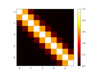
Now, given our covariance function, we can apply it to all pair combinations to make the covariance matrix (represented as a heat map here):

Matrix from the covariance function

then we invert it (after we add some noise to the diaganol to ensure it's not ill-conditioned):

Inverted matrix of the covariance function

then element-wise multiply it with the observed y(x) values (ie, all those corresponding to x in the range 1 to 10):

Alpha

This completes the training process.

Now, all the Figaro example does is plug these tensors into pre-packaged formulas for the expected value (μ_*) and covariance matrix (Σ_*) of the derived Gaussian. These can be found in Kevin Murphy's excellent "Machine Learning: a Probabilistic Perspective", equations 15.8 and 15.9: 

μ_* = μ(X_*) + K_*^TK^-1(f - μ(X))
Σ_* = K_** - K_*^TK^-1K_* 

where

X is the observed data

f is the mapping from the known inputs (X) to outputs

X_* is the data for which we wish to predict f 

K is the observed data that has gone through the kernel function/covariance matrix and is a function of  (X, X)

K_* is a mix of the data X and X_* that has gone through the kernel function/covariance matrix and is a function of  (X, X_*)

K_** is the data X_* that has gone through the kernel function/covariance matrix and is a function of  (X_*, X_*)

The derivation of these equations is beyond me, as is why the Figaro demo uses 1000 iterations when I get similar results with 1 or 10 000.

Next time. In the meantime, it appears that Murphy's book is going to be available online in a year's time and the code is already being translated to Python and can be found at GitHub here.

Further reading 

Gaussian Processes for Dummies [Kat Bailey's Blog]

The Model Complexity Myth [Jake VanderPlas's Blog]