3D Plots

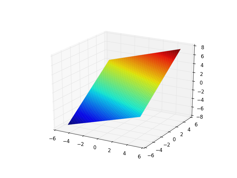
I'm creating a Spark linear algebra library but wanted to plot a few graphs to get an idea of what's going on. These are the tools I tried.

Sympy

Sympy looked good as it allowed implicit functions. For instance, you can write:

from sympy import symbols
from sympy.plotting import plot3d

x, y = symbols('x y')

p = plot3d((x/2) + y, (x, -5, 5), (y, -5, 5))

and get the plane that represents z = (x/2) + y.

The problem was that "SymPy uses Matplotlib  behind the scenes to draw the graphs" [1] and Matplotlib has some issues in the z-order while rendering.

So, although SymPy gives you a lot more than just plotting, I moved on to...

Mayavi

... which renders things beautifully.

Until I tried to do something clever.

First, I had to update pip. Then, with, I tried:

from mayavi import mlab
.
.
mlab.options.backend = 'envisage'

which gave me:

ImportError: No module named envisage.ui.workbench.api

And after some googling, it looked like I needed to mess around with all sorts of libraries so I was a coward and gave up quickly.

Jzy3d

It turns out that there is a perfectly good Java library called Jzy3d which is quite mature.

Given:

v₁ = [8, -2, 2]
v₂ = [4,  2, 4]

I wanted to plot these vectors, the surface on which they lie and the shortest distance between this plane and [5, -5, 2] (this exercise can be found in Philip Klein's excellent "Coding the Matrix").

First, I had to convert this information to something Jzy3d can handle - which looks like this:

        Mapper plane = new Mapper() {
            @Override
            public double f(double x, double y) {
                return (x + (2 * y)) / 2;
            }
        };

that is, we first need to turn these vectors into an implicit function. Well, any point (x, y, z) on the plane can be described as s v₁ + t v₂ where s and t are any real numbers. Turning this information into parametric equations is easy:

x = 8s  + 4t
y = -2s + 2t
z = 2s  + 4t

and solving these simultaneous equations gives us the implicit function:

x + 2y - 2z = 0

or

z = (x + (2 * y)) / 2

which is the equation we find in our Java code above.

Finding the normal to an implicit function is simply the coefficients, that is [1, 2, -2]. At the point the normal meets [5, -5, 2] (which we'll call b) is the point where u b =s v₁ + t v₂. Once again, convert to parametric equations and then solve the simultaneous equations and you'll find t=-0.5 and s=1. This will give the point [6, -3, 0] and Jzy3d renders it like this:

where the red line is the normal, the green line is the point and the blue line is the closest point on the surface.

The rendering can be a bit jagged and I need to look at adding arrows to the vectors but so far, this seems to be the easiest plotting library to use.

[1] Doing Math with Python (No Starch Press)