The Joy of Sets?

The standard Scala Set violates basic algebra. Let's take two sets, x and y:

@ val x = Set(1, 2, 3) 

x: Set[Int] = Set(1, 2, 3)

@ val y = Set(3, 2, 1) 

y: Set[Int] = Set(3, 2, 1)

@ x == y 

res2: Boolean = true

If they're equal, we should be able to substitute one for another. Let's see how that goes:

@ def giveHead(s: Set[Int]): Int = s.head 

defined function giveHead

@ giveHead(x) 

res6: Int = 1

@ giveHead(y) 

res7: Int = 3

So, I get different results depending on which of two equal objects I call the method - crazy. 

topkek

Isn’t Map.toList impure or something like that?

tpolecat

It's pure but non-congruent with equality. m1 === m2 doesn't imply m1.toList === m2.toList because they could differ in their iteration order. That's why it's not Foldable. You can get those instances from alleycats I believe.

The unordered business is there to guarantee that Eq and Foldable are congruent (i.e., that a === b implies a.toList === b.toList) which is not necessarily true of data types like Set and Map: these are only UnorderedFoldable which requires you to fold into a commutative monoid which destroys any information you might get from observing iteration order. Which is to say "unordered" doesn't necessarily say anything about execution order, it just says any ordering that might be there won't be observable. 

Although often forgotten, sets are not functors.

You cannot parTraverse a Set (or Maps) in Cats. It just won't compile. This is a property of that particular data structure but it's not limited to Sets:

Fabio Labella @SystemFw Nov 16 16:55

You cannot traverse an [FS2] Stream, because it implies it's finite. Look at evalMap instead if the use case is "evaluate an action on each element". 

Instead, you must parUnorderedTraverse a Set.

Adam Rosien @arosien Nov 10 20:17

every Traverse is also an UnorderedTraverse, so they should act the same in that case (and since every CommutativeApplicative is also an Applicative, you can still call unorderedTraverse on something that has a Traverse)

To traverse a set (albeit unordered), the UnorderedTraverse will put the Set into a higher kinded type G[_]. If we want to take advantage of this say for List[_], we need a concrete implementation of a Parallel[List]. Among other things, this defines how to map from List[_] to Set[_] and back again. This brings us back to the problems with set's toList function - but at least now we're explicit in how we want this handled. 

Yet more Spark tips

Backfilling

You can use inline or inline_outer (the latter outputting nulls [SO]) to explode an array of structs into a table [PySpark docs]. Combined with sequence, you can generate new rows. This is very useful for backfilling data. 

Leveraging this StackOverflow answer, I could backfill data with this Spark SQL:

inline_outer(
    transform(
        sequence(0,
                 int(datediff(2022-10-23, END_DATE)),
                 7), 
        i -> (date_add(END_DATE, i) as EVENT_DATE,
              IF(i=0, Y, YHAT) as YHAT)
    )
)

This would create new rows for each week (7) beween a date in column END_DATE and 23 October 2022. For each row we generate, we get that date and a value Y if it's the first new date or YHAT if not.

Combine this with the columns we want fixed with:

    df = df.selectExpr(LIST_OF_COLUMNS + [SQL_STRING_ABOVE])

The keyword transform maps elements in an array using a user-defined function [docs]. The array can be generated by sequence which simply generates an array of elements that have typesafety - that is, if you were adding a sequence of integers to a date, it will yield increasing dates.

Reading RDBMS from Spark

Spark defaults to one JVM reading the data from a call to an RDBMS. It cannot possibly know how to divide the work a priori. However, you can get it to partition the workload if you tell it how - see here. 

Skew

Skew can now be autohandled apparently (see the Spark docs) since version 3.0.

Partitions and OOMEs

You don't need to just call .collect() to see:

org.apache.spark.SparkException: Job aborted due to stage failure: Total size of serialized results of 16 tasks (1024.1 MB) is bigger than spark.driver.maxResultSize (1024.0 MB)

This can happen when there are too many partitions [StackOverflow] and the amount of metadata overwhelms the driver. The solution is to use fewer partitions or add more driver memory.

Further notes on diagnosing this can be found in a previous post here.

PyArrow does not come as standard

"Pandas UDFs are user defined functions that are executed by Spark using Arrow to transfer data and Pandas to work with the data, which allows vectorized operations. A Pandas UDF is defined using the pandas_udf as a decorator or to wrap the function, and no additional configuration is required. A Pandas UDF behaves as a regular PySpark function API in general." [Spark docs] 

However, in Palantir's Foundry, this code gives:

  File "/myproject/datasets/_PH_Test.py", line 12, in test_ph
    @pandas_udf("col1 string, col2 long")
  File "/scratch/asset-install/6add7b36ad350d9f0c07885622f2e3ae/miniconda36/lib/python3.6/site-packages/pyspark/sql/pandas/functions.py", line 332, in pandas_udf
    require_minimum_pyarrow_version()
  File "/scratch/asset-install/6add7b36ad350d9f0c07885622f2e3ae/miniconda36/lib/python3.6/site-packages/pyspark/sql/pandas/utils.py", line 56, in require_minimum_pyarrow_version
    "it was not found." % minimum_pyarrow_version) from raised_error
ImportError: PyArrow >= 1.0.0 must be installed; however, it was not found.

Locally, trying to install it initially met with failure:

$ pip install pyarrow
...
    CMake Error at /home/henryp/Downloads/Temp/cmake-3.23.1-linux-x86_64/share/cmake-3.23/Modules/FindPackageHandleStandardArgs.cmake:230 (message):
      Could NOT find Arrow (missing: ARROW_INCLUDE_DIR ARROW_LIB_DIR
      ARROW_FULL_SO_VERSION ARROW_SO_VERSION)
...

Upgrading pip solved that one (pip install --upgrade pip)

Comparing Time Series

The domain

Given a time series of various metrics for various hospitals in a region, I want to find if there is any correlation between them. Specifically, I am interested in any metric for one hospital where another lags behind it by a day or so.

Initially, my results were great. In fact, they were too good to be true. See, the problem is that hospital metrics all dance to the same tune of time. When you take away the noise, there is a regular weekly rhythm to the stats.

Consequently, it was not a case of one metric predicting another. It was more that both were conforming to a weekly pattern. This was true even when we considered lags between the two series.

For instance, there may be systemic bias at play. In this case, inpatients are often eagerly discharged in time for the weekend when there are fewer staff on duty. This is true for all hospitals nationally so we should not assume somehow one hospital has some unspecified influence on another if we see them both behaving in the same manner.

In the case of a lag, Mondays see a sharp rise in patients so we should not take too seriously an (anti) correlation with the previous Friday at another hospital.

The importance of being startionary

The problem we had was that our time series was not startionary. "Making a distribution stationary is a strict requirement in time series forecasting... If a distribution is not stationary, then it becomes tough to model." [BexT, TowardsDataScience]

But what does it mean to be stationary?

Terminology

"A stationary time series is one whose properties do not depend on the time at which the series is observed. Thus, time series with trends, or with seasonality, are not stationary — the trend and seasonality will affect the value of the time series at different times. On the other hand, a white noise series is stationary — it does not matter when you observe it, it should look much the same at any point in time." [Forecasting: Princples and Practice a free, online book]

Note that just because a time series looks highly cyclical to the eye, it doesn't mean it is. If you can't predict where it will be in 10 years, it is stationary.

Example of highly cyclical, non-stationary data: annual sales that are heavily influenced by Christmas.

Example of highly cyclical, stationary data: the population of foxes and rabbits. Although cyclical, the exact length of a cycle is not known.

"The [200 day] Google stock price was non-stationary ... but the daily changes were stationary ... This shows one way to make a non-stationary time series stationary — compute the differences between consecutive observations. This is known as differencing.

"Transformations such as logarithms can help to stabilise the variance of a time series. Differencing can help stabilise the mean of a time series by removing changes in the level of a time series, and therefore eliminating (or reducing) trend and seasonality." [ibid]

The Tools

How do we know that our series is stationary? Jason Brownlee [TowardsDataScience] suggests three approaches: look at plots, use statistical tests or compare summaries for partitions of the data. I'll look at the first two.

When we plot our data, it certainly doesn't look like it is stationary at first blush as there seem regular troughs and peaks:

A&E admissions at two hospitals

If we zoom in, we can see there is a definite weekly cycle:

Zoomed in, plus the 1st order derivatives

One trick to make the series stationary is to use the first order derivatives of the data instead of the actual data itself. However, this too seems to be non-stationary (see pic above).

To check more rigorously if the series is stationary, we can use the Augmented Dickey-Fuller test in StatsModels. Here, the null hypothesis is the distribution is non-stationary, time-dependent. The p-value of us rejecting the null hypothesis was about 0.02 for the raw data and 7x10^-9  and 8x10^-21 for the first and second derivatives respectively. 

But the data and its derivatives still look stationary to me (why these ADF tests reported such low p-values is still a mystery to me). Some Fourier analysis seems to suggest that the data is indeed time-dependent:

Fourier analysis of the admissions data

Look at those peaks at about 0.14 (= 1/7) on the x-axis that indicate a weekly trend.

Another way to make the data stationary is to center the data. We know how to do this with hospitals as admissions are strongly correlated with days of the week. After doing this, the Fourier analysis looks like:

Fourier analysis on the same admissions centered of their mean by day-of-week

Much better! The largest Augmented Dickey-Fuller values is 2x10^-7 and the timeseries of centered data also looks more likely to be stationary:

The centered admissions data for two nearby hospitals

Now, we can run a Granger Causality test. Here "we reject the null hypothesis that x₂ does not Granger cause x₁ if the p-values are below a desired size of the test." [StatsModels docs].

Conclusion

Granger Causality comes with caveats, one of which is that your data is stationary. A reason why this is the case is that making your data stationary avoids confounding factors that cause spurious relationships [Wikipedia].

To make your time series stationary may require some domain knowledge.

Diagnosing Spark Docker issues

I'm trying to talk on my host machine to a docker container running Spark. Unfortunately, upon connection I see:

Caused by: java.lang.RuntimeException: java.io.InvalidClassException: org.apache.spark.rpc.netty.RpcEndpointVerifier$CheckExistence; local class incompatible: stream classdesc serialVersionUID = 5378738997755484868, local class serialVersionUID = 7789290765573734431

This appears to be something of a known issue with this container.

We get the client code's classpath using SBT [SO]: 

sbt "export runtime:fullClasspath"

and taking the classpath for my module, we run:

serialver -classpath $FROM_ABOVE org.apache.spark.rpc.netty.RpcEndpointVerifier\$CheckExistence

which yields:

org.apache.spark.rpc.netty.RpcEndpointVerifier$CheckExistence:    private static final long serialVersionUID = 5378738997755484868L;

(The error message is coming from Spark master).

On the host, we login to the master container with:

docker exec -it $(docker ps | grep spark-master:3.2.1 | awk '{print $1}') /bin/bash

where we run:

for FILE in $(find spark/jars/) ; do { echo $FILE ; unzip -l $FILE | grep CheckExistence ; } done

and discover the class is in spark/jars/spark-core_2.12-3.2.1.jar. Hmm, the name suggests this Docker container has a Spark instance built with Scala 2.12 and I'm using Scala 3 which is compatible with 2.13 but not (apparently) 2.12.

Mounting the host file system from the container:

docker run -it -v /tmp:/mnt/disk bde2020/spark-master:3.2.1-hadoop3.2 /bin/bash

I copied all the Spark jars to a temporary folder. Then on the host:

CP="" ; for JAR in $(ls /tmp/jars/*.jar) ; do { CP="$CP:$JAR" ; } done

serialver -classpath $CP org.apache.spark.rpc.netty.RpcEndpointVerifier\$CheckExistence

yielded 7789290765573734431L.

So, at this point it appears I am SooL and need to get a new container.

Spark and Pandas

It seems that not just the PySpark driver but also the Spark JVM workers spawns Python daemons (see Obi Orciuch's blog)

Spark keeps a track of Python processes (source). In PythonWorkerFactory we read: "Because forking processes from Java is expensive, we prefer to launch a single Python daemon, pyspark/daemon.py (by default) and tell it to fork new workers for our tasks. This daemon currently only works on UNIX-based systems now because it uses signals for child management, so we can also fall back to launching workers, pyspark/worker.py (by default) directly. "

Indeed, running:

$SPARK_HOME/sbin/start-all.sh
$SPARK_HOME/bin/pyspark  --master=spark://127.0.1.1:7077

and then running in this shell:

something = 'hello ' * 1000000
another_string = spark.sparkContext.parallelize(something)
another_string.map(lambda a: a.upper()).take(100)

During all this, if you run:

watch -d "ps -ef | grep -i python | grep -v ps | grep -v grep"

you'll see a Python instance stared when the PySpark shell but also something like "python3 -m pyspark.daemon". If you find the parent of this process, you'll find it's a Java process called "CoarseGrainedExecutorBackend". This is a cluster worker.

Indeed, if you accidentally use a different Python version in your driver as your workers (the workers will default to the system's version of Python), you'll see errors like this:

Exception: Python in worker has different version 3.6 than that in driver 3.9, PySpark cannot run with different minor versions. Please check environment variables PYSPARK_PYTHON and PYSPARK_DRIVER_PYTHON are correctly set.

"Note that all data for a group will be loaded into memory before the function is applied. This can lead to out of memory exceptions, especially if the group sizes are skewed. The configuration for maxRecordsPerBatch is not applied on groups and it is up to the user to ensure that the grouped data will fit into the available memory." (Spark docs)

Also note that Wes McKinny, author of Pandas, notes "my rule of thumb for pandas is that you should have 5 to 10 times as much RAM as the size of your dataset" (albeit in 2017). 

The applyInPandas function is the gateway for Pandas in PySpark but be warned. "This function requires a full shuffle. All the data of a group will be loaded into memory, so the user should be aware of the potential OOM risk if data is skewed and certain groups are too large to fit in memory." (Spark docs)

There is some nice documentation here but theSpark code that passes the Python process all it needs is here in GitHub.

More ML pipeline debugings

The simpler model is sometimes better. 

We used Meta's Prophet to forecast the flow of patients between care providers. However, we had problems. 

First, the errors were pretty high when back testing. The average error over all care providers was about 20%.

Second, the sum of all care providers in a region was sometimes wildly larger than we'd expect. Curiously, the forecasts for the individual providers in the region were reasonably good.

Thirdly, even if the total numbers of patients flowing between care providers were plausible, it wasn't compatible with the model that forecast the number of patients at the care provider.

A simpler model

We tried a model that used just the historical average number of patients for a care provider. This calculation was over all data on the same day of the week and same month of the year (but ignoring the Covid pandemic when figures were weird).

Example: for any given Monday in January, we simply looked at the average flow between two nodes for all Mondays in every January over all non-Covid years. 

This approach yielded a lower error than Prophet - about 16%. See below for what metric we used to quantify the error. 

Odd figures

When we rendered the Prophet forecasts in the front-end application, they didn't seem too bad most of the time. For instance, we predict that 3027 people would go through the emergency departments in all hospitals in region X tomorrow when today it was 2795. OK, not too shocking.

But if we looked at flows with small numbers, the figures looked crazy. For instance, we predicted the number of people being discharged from all hospitals in a region into mental health units would be 15 tomorrow when this week it had actually averaged about 1.

One of the issues was Prophet itself. Prophet timeseries for small numbers may well have predictions below 0. Obviously, the users did not like us predicting a negative number of patients. But if we simply mapped all negative number to zero, we might get surprises.

Let's take some random numbers:

>>> import numpy as np 
>>> xs = np.random.normal(1, 2, 10)
>>> sum(xs)
9.788255911110234

but:

>>> gt0 = lambda x: 0 if x<0 else x

>>> sum(list(map(gt0, xs)))

12.020263767841016

The forecast for individual care providers was considered good even though Prophet would regularly predict, say, 1 person being sent from an emergency department to mental health facilities when often the figure was actually zero. 

But this 100% error was operationally fine for the clinicians because it was such a small number. It only became an issue when summed over all providers in the region. 

Absent data

We thought using the simpler, historical averages would solve this problem but it didn't. So, we took a closer look at the data. An emergency department would only discharge people into a mental health unit roughly once a week. In the absence of such a discharge, there would be no record. Why should there be? The hospitals only record events that happen not events that don't.

For both Prophet and historical averages, we're not feeding information into our model. But the absence of data is itself information! For instance, the averages of two series are different if you choose to ignore zeros:

>>> np.mean([5,0,0,0,0,3,0,0])

1.0

>>> np.mean([5,3])

4.0

Not a revelation when you think about it but backfilling this information via Spark was a bit gnarly. This StackOverflow answer helped. Once we did this, all figures agreed.

Vertices and Edges

Using historical data, the average flows between nodes necessarily summed to the values at the nodes. This was not true for independent Prophet models.

Imagine we have three care providers a, b and c. 

The number of patients that daily flow through them are A, B and C respectively.

Patients flow from a to c and from b to c.
Let's say the flow from a to c is X and the flow from b to c is Y.

The expected number of patients flowing through c is therefore exactly:

E[C] = E[X+Y] = E[X] + E[Y]  

Compare this to Prophet (or any other model that takes just the historical C to forecast future C). In general:

E[C] != E[A] + E[B]

This is important at the front-end where users are complaining that the predicted flows on their screen don't add up.

Which error metric to use?

I was using root mean squared error to calculate errors whereas a colleague was using  mean absolute error. Which is most appropriate must be decided on a case by case basis. RMSE punishes a data set with a large number of outliers. Whereas, "If being off by 10 is just twice as bad as being off by 5, then MAE is more appropriate". Note that "MAE will never be higher than RMSE because of the way they are calculated" - see this SO answer.

Conclusion

Start with the simplest model you can. It's generally easier to implement, cognitively less demanding and chances are that it will give reasonable results anyway. If the results are not good enough, only then investigate shiny new toys.

Time series

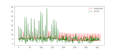
Meta's much hyped Prophet seems to have problems identifying spikes in small numbers. For instance, we had a hospital that was admitting 4- to 5-times the normal number of patients on Fridays. Then, one day for whatever reason, Friday became a day like any other. Despite a lot of brute-force hyperparameter tuning, the ratio of RMSE/mean stayed at about 0.69.

Prophet (mis)handling significant behavioural change

From the issues on Github, "by default the model will do a bad job on this time series because the model assumes smooth seasonality. That assumption comes because seasonality is modeled with a truncated Fourier series, which basically means it cannot change very rapidly."

You can add_regressors to the model but firstly I don't want to manually do this (I'd have to inspect thousands of data sets by-eye!) and when I tried it, my RMSE was worse - for reasons as yet unknown. Plots showed that it simply translated predictions for that spline down the y-axis; there was not change in how it treated the periodicity.

SARIMAX

On the same data, the default SARIMAX implementation in StatsModel gives you:

SARIMAX with default values

You need to explicitly tell it that there is weekly seasonality. In this  case seasonal_order = (1, 0, 1, 7) works well. Note that 7 means we expect weekly behaviour. Indeed, SARIMAX quickly recognises the change:

SARIMAX with an explicitly provided seasonality

And the overall RMSE/mean ratio becomes a little better at 0.61.

Correlations

Don't be fooled by in-series correlations versus cross-series correlations. This SO link shows how the random walk generated by the tossing of two coins can appear to be correlated (just by luck) when of course they could not possibly be. This is because each have in-series correlation; each value in the cumulative total of HEADS-TAILS will be +/-1 the previous.

SciPy appears to have a tool to find the correlation between series even if the effect is lagged.